Calculate the Total Value of the Filtered List in Excel

Calculate the Total Value of the Filtered List in Excel covers the essential facts behind the topic, including what changed, why it mattered, and how it affected users.

• MS Excel 2007 - Lesson 8: Sort and Filter

The tutorial is implemented in Excel 2003, which is quite old, but you can still apply this calculation on newer Excel versions such as Excel 2007, Excel 2010, Excel 2013, Excel 2016, because of the user guide Excel Subtotal function.

The figure below shows a filtered list. You can look at the column on the left and notice that many rows are not displayed because the filter is not satisfied.

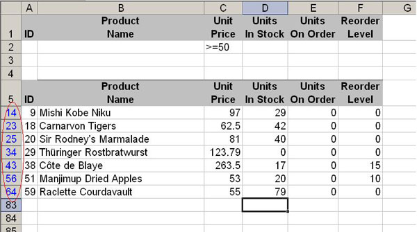
The next figure shows you the results when we try to calculate the total value with the SUM () function.

At first glance, it is easy to see incorrect results: the total value is too large, why? That's because the SUM () function calculates all values ??from D14 to D64, not just summing the filtered values. There is no way for the SUM () function to know that we want to exclude values ??that do not satisfy the filter.

The solution to this problem is very simple. Just click AutoSum, Excel will automatically call SUBTOTAL () instead of SUM (). This function will look at the entire list from D6 to D82 but only calculate the total value of the filter match.

About Subtotal ()

The SUBTOTAL () function will look at the entire list of values ??in column D and only calculate the filter match values. You can look at the image above and guess that it is thanks to declaring argument 9. However, this argument tells Excel that we want to calculate TOTAL reference values. The following table lists accepted arguments:

Including hidden values

Ignore hidden values

Jaw

First

101

AVERAGE ()

2

102

COUNT ()

3

103

COUNTA ()

4

104

MAX ()

5

105

MIN ()

6

106

PRODUCT ()

7

107

STDEV ()

8

108

STDEVP ()

9

109

SUM ()

Ten

110

VAR ()

11

111

VARP ()

After looking at the table above, you are probably wondering the difference between 9 and 109. When we use argument 9, SUBTOTAL () will sum the hidden values. When we use argument 109, SUBTOTAL () will ignore hidden values. We need to distinguish the hidden value and the value that is removed due to not satisfying the filter. Hiding a row can be done by right-clicking on the row order then selecting Hide. This is completely different from the rows that are not displayed because the filter is not satisfied.

• How to use the Power function in Excel
• How to use the Round function in Excel
• How to use Vlookup function in Excel