Complete tutorial of Excel 2016 (Part 6): Change the size of columns, rows and cells

The following article shows you some ways to change the size of columns, rows, and cells in Excel 2016. Please refer!

By default, each row and each column of a new spreadsheet will have the same height and width. Excel 2016 allows you to adjust row and column widths in different ways, including wrapping text and merging cells .

See the video below to learn more about how to change column, row, and cell sizes in Excel 2016 :

Instructions for Excel 2016 part 6:

1. Adjust the width of the Excel 2016 column
2. Adjust the width of Excel columns automatically with AutoFit
3. Adjust height of Excel 2016 rows
4. Edit all rows or Excel 2016 columns
5. Insert, delete, move and hide rows, Excel 2016 columns
   1. I. To insert goods
   2. II. To insert a column:
   3. III. To delete rows or columns:
   4. IV. To move rows or columns:
   5. V. To hide and unhide rows or columns:
7. Break lines and merge Excel 2016 cells
   1. I. Breaking lines in Excel cells:
   2. II. Merge cells with the Merge & Center command:
   3. III. Access to many integration options:
   4. IV. Choose center:

Adjust the width of the Excel 2016 column

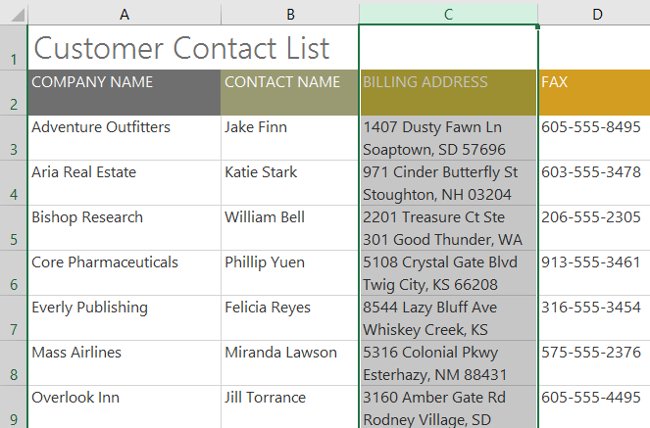
In the example below, column C is too narrow to display all the content in the cells. We can make all this content visible by adjusting the width of column C.

1. Move the mouse over the column row in the column header so that the cursor becomes a double arrow.

Complete tutorial of Excel 2016 (Part 6): Change the size of columns, rows and cells Picture 1

2. Click and drag the mouse to increase or decrease the column width.

Complete tutorial of Excel 2016 (Part 6): Change the size of columns, rows and cells Picture 2

3. Release the mouse. The column width will be changed.

Complete tutorial of Excel 2016 (Part 6): Change the size of columns, rows and cells Picture 3

1. With numeric data, the cell displays the pound sign (#######) if the column is too narrow. Simply increase the column width to make the data visible.

Adjust the width of Excel columns automatically with AutoFit

The AutoFit feature allows you to set the width of the column to match its content.

1. Move the mouse to the upper part of the column line in the column header so that the cursor becomes a double arrow.

Complete tutorial of Excel 2016 (Part 6): Change the size of columns, rows and cells Picture 4

2. Double click. The column width will be changed automatically to match the content.

Complete tutorial of Excel 2016 (Part 6): Change the size of columns, rows and cells Picture 5

1. You can also use AutoFit to automatically adjust the width for multiple columns at once. Simply select the columns you want AutoFit, then select the AutoFit Column Width command from the Format drop-down menu on the Home tab. This method can also be used for row height.

Complete tutorial of Excel 2016 (Part 6): Change the size of columns, rows and cells Picture 6

Adjust height of Excel 2016 rows

1. Move the mouse to the row so that the cursor becomes a double arrow.

Complete tutorial of Excel 2016 (Part 6): Change the size of columns, rows and cells Picture 7

2. Click and drag the mouse to increase or decrease the row height.

Complete tutorial of Excel 2016 (Part 6): Change the size of columns, rows and cells Picture 8

3. Release the mouse. The height of the selected item will be changed.

Complete tutorial of Excel 2016 (Part 6): Change the size of columns, rows and cells Picture 9

Edit all rows or Excel 2016 columns

Instead of changing each row and column size individually, you can change the height and width of each row and each column at the same time. This method allows you to set a uniform size for each row and column in the spreadsheet. In the example, we will set the row height.

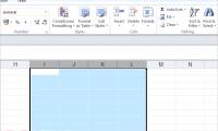
1. Locate and click the Select All button just below the name box to select each cell in the spreadsheet.

Complete tutorial of Excel 2016 (Part 6): Change the size of columns, rows and cells Picture 10

2. Move the mouse over the row row so that the cursor becomes a double arrow.

3. Click and drag the mouse to increase or decrease the row height, then release the mouse when satisfied. The row height will be changed for the entire spreadsheet.

Complete tutorial of Excel 2016 (Part 6): Change the size of columns, rows and cells Picture 11

Insert, delete, move and hide rows, Excel 2016 columns

After working with a spreadsheet for a period of time, you may find that you want to insert new columns or rows, delete certain rows or columns, move them to another location in the spreadsheet or even hide them.

I. To insert goods

1. Select the row title below where you want the new item to appear. In this example, we want to insert a row between rows 4 and 5 , so we will select row 5 .

Complete tutorial of Excel 2016 (Part 6): Change the size of columns, rows and cells Picture 12

2. Click the Insert command on the Home tab.

Complete tutorial of Excel 2016 (Part 6): Change the size of columns, rows and cells Picture 13

3. New row will appear above the selected row.

Complete tutorial of Excel 2016 (Part 6): Change the size of columns, rows and cells Picture 14

1. When inserting new rows, columns or cells, you will see a brush icon next to the inserted cells. This icon allows you to choose how to format Excel cells. By default, Excel formats insert rows of the same format as the cells in the row above. To access more options, hover over the icon, then click the drop-down arrow.

Complete tutorial of Excel 2016 (Part 6): Change the size of columns, rows and cells Picture 15

II. To insert a column:

1. Select the column header to the right where you want the new column to appear. For example, if you want to insert a column between columns D and E, select column E.

Complete tutorial of Excel 2016 (Part 6): Change the size of columns, rows and cells Picture 16

2. Click the Insert command on the Home tab.

Complete tutorial of Excel 2016 (Part 6): Change the size of columns, rows and cells Picture 17

3. The new column will appear on the left of the selected column.

Complete tutorial of Excel 2016 (Part 6): Change the size of columns, rows and cells Picture 18

1. When inserting rows and columns, make sure you select the entire row or column by clicking on the title. If you select only one cell in the row or column, the Insert command only inserts a new cell.

III. To delete rows or columns:

It's easy to delete rows or columns that you no longer need. In the example, we will delete a row, but you can also delete a column this way.

1. Select the item you want to delete. In the example, we will choose row 9 .

Complete tutorial of Excel 2016 (Part 6): Change the size of columns, rows and cells Picture 19

2. Click the Delete command on the Home tab.

Complete tutorial of Excel 2016 (Part 6): Change the size of columns, rows and cells Picture 20

3. The selected item will be deleted and the rows around it will change. In the example, row 10 has moved up to row 9.

Complete tutorial of Excel 2016 (Part 6): Change the size of columns, rows and cells Picture 21

1. It is important that you understand the difference between deleting rows or columns and only deleting its contents. If you want to remove content from a row or column without making another row or column change, right-click a title, then select Clear Contents from the drop-down menu.

Complete tutorial of Excel 2016 (Part 6): Change the size of columns, rows and cells Picture 22

IV. To move rows or columns:

Sometimes you may want to move a column or row to reorder the contents of the spreadsheet. In the example, we will move a column, but you can move a row in the same way.

1. Select the desired column title for the column you want to move.

Complete tutorial of Excel 2016 (Part 6): Change the size of columns, rows and cells Picture 23

2. Click the Cut command on the Home tab or press Ctrl + X on the keyboard.

Complete tutorial of Excel 2016 (Part 6): Change the size of columns, rows and cells Picture 24

3. Select the column header to the right where you want to move the column. For example, if you want to move a column between columns E and F, select column F.

Complete tutorial of Excel 2016 (Part 6): Change the size of columns, rows and cells Picture 25

4. Click the Insert command on the Home tab, then select Insert Cut Cells from the drop-down menu.

Complete tutorial of Excel 2016 (Part 6): Change the size of columns, rows and cells Picture 26

5. The column will be moved to the selected position and the surrounding columns will change.

Complete tutorial of Excel 2016 (Part 6): Change the size of columns, rows and cells Picture 27

1. You can also access Cut and Insert commands by right-clicking and selecting the desired command from the drop-down menu.

Complete tutorial of Excel 2016 (Part 6): Change the size of columns, rows and cells Picture 28

V. To hide and unhide rows or columns:

Sometimes, you may want to compare certain rows or columns without changing the way the spreadsheet is organized. To do this, Excel allows you to hide rows and columns if needed. In the example, we will hide some columns, but you can hide the rows in the same way.

1. Select the column you want to hide, right-click, then select Hide from the format menu. In the example, we will hide columns C, D and E.

Complete tutorial of Excel 2016 (Part 6): Change the size of columns, rows and cells Picture 29

2. The columns will be hidden. The green column shows the location of the hidden columns.

Complete tutorial of Excel 2016 (Part 6): Change the size of columns, rows and cells Picture 30

3. To unhide the columns, select the columns on both sides of the hidden column. In the example, we will select column B and F. Then right-click and select Unhide ( Unhide ) from the format menu.

Complete tutorial of Excel 2016 (Part 6): Change the size of columns, rows and cells Picture 31

4. The hidden columns will be displayed again.

Complete tutorial of Excel 2016 (Part 6): Change the size of columns, rows and cells Picture 32

Break lines and merge Excel 2016 cells

Whenever there is too much cell content displayed in a cell, you can decide to break the line or merge the cells again instead of resizing a column. Line breaks automatically modify the row height of the cell, allowing the cell content to be displayed on multiple lines. Including cells allows you to combine a cell with empty cells to create a large cell.

I. Breaking lines in Excel cells:

1. Select the cells you want to interrupt. In this example, we will select the cells in column C.

2. Click the Wrap Text command on the Home tab.

Complete tutorial of Excel 2016 (Part 6): Change the size of columns, rows and cells Picture 33

3. The text in the selected cells will be interrupted.

Complete tutorial of Excel 2016 (Part 6): Change the size of columns, rows and cells Picture 34

1. Click the Wrap Text command again to extract the text.

II. Merge cells with the Merge & Center command:

1. Select the range you want to merge. In the example, we will select the range A1: F1 .

2. Click the Merge & Center command on the Home tab.

Complete tutorial of Excel 2016 (Part 6): Change the size of columns, rows and cells Picture 35

3. The selected cells will be merged again and the text will be centered.

Complete tutorial of Excel 2016 (Part 6): Change the size of columns, rows and cells Picture 36

III. Access to many integration options:

If you click the drop-down arrow next to the Merge & Center command on the Home tab, the Merge drop-down menu will appear.

Complete tutorial of Excel 2016 (Part 6): Change the size of columns, rows and cells Picture 37

From here, you can choose:

1. Merge & Center: merge selected cells into one cell and center text;
2. Merge Across : merge selected cells into larger cells while keeping each row separate;
3. Merge Cells : merge selected cells into one cell but not between text;
4. Unmerge Cells : unmerge the selected cells.

You will have to be careful when using this feature. If you merge multiple cells that contain data, Excel will only retain the contents of the upper left cell and remove other content.

IV. Choose center:

Merge can be useful for organizing your data, but it can also create problems later. For example, it may be difficult to move, copy and paste content from merged cells. A good option to merge is the Center Across Selection , creating a similar effect without actually merging the cells.

1. Select the desired range of cells. In the example, we select the range A1: F1.

1. Note: If you have merged these boxes, you should un-merge them before continuing to step 2 .

2. Click the small arrow in the lower right corner of the Alignment group on the Home tab.

Complete tutorial of Excel 2016 (Part 6): Change the size of columns, rows and cells Picture 38

3. A dialog box will appear. Locate and select the Horizontal drop-down menu, select Center Across Selection , then click OK .

Complete tutorial of Excel 2016 (Part 6): Change the size of columns, rows and cells Picture 39

4. The content will be centered on the selected cell range. As you can see, this produces the same visual result as merging and centering, but it preserves each cell inside the range A1: F1 .

Complete tutorial of Excel 2016 (Part 6): Change the size of columns, rows and cells Picture 40

Having fun!

Micah Soto

Update 25 May 2019