Excel 2016 - Lesson 8: How to format numbers in Excel (Number Formats)

When you import the data in an Excel spreadsheet, it always defaults to General format so that Excel formats can display and calculate the correct format of the actual data. You need to set the format. for it. Let's learn about Number Formats with TipsMake.com in Excel 2016!

Format numbers in Excel

Whenever working with spreadsheets, it's better to use number formats that are appropriate for your data. Number formats indicate the exact data type you are using in the spreadsheet, such as percentage (%), currency ($), timestamps, dates, etc.

Watch the video below to learn more about Number Formats in Excel:

Why use number format?

Formatting numbers in Excel not only makes your spreadsheet easier to read, but it also makes it easier to use. When you apply a number format, you are telling the spreadsheet exactly what type of value is stored in a cell. (For example, the date format tells the spreadsheet that you are entering a specific calendar date .) This allows the spreadsheet to better understand the data, helping to ensure data and formula consistency is maintained. Yours is calculated correctly.

If you don't need to use a specific number format, the spreadsheet will usually apply the general number format by default. However, the global format may apply some minor formatting changes to your data.

Apply number formatting

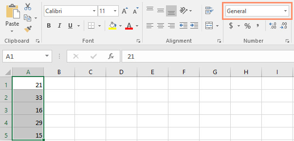
Just like other types of formatting, such as changing font color, you apply number formats by selecting cells and selecting the desired formatting options. There are two main ways to choose a number format:

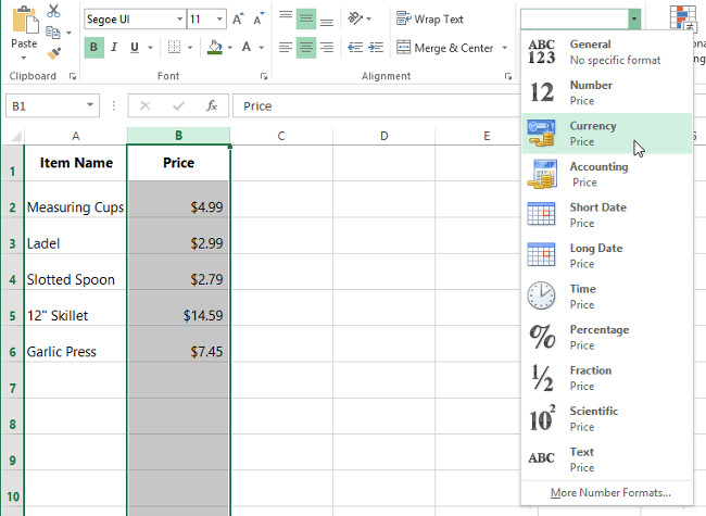
1. Go to the Home tab , click the Number Format drop-down menu in the Number group , and select the desired format.

Excel 2016 - Lesson 8: How to format numbers in Excel (Number Formats) Picture 1

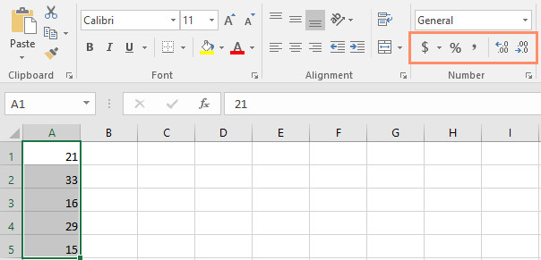
1. You can click one of the quick number format commands below the drop-down menu.

Excel 2016 - Lesson 8: How to format numbers in Excel (Number Formats) Picture 2

Alternatively, you can also select the desired cells and press Ctrl + 1 on the keyboard to access other number formatting options.

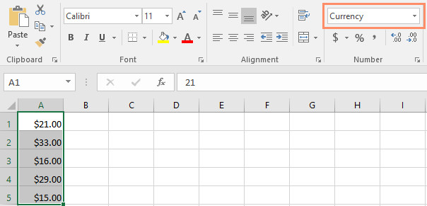
In this example, we've applied the Currency number format to add a currency symbol ($) and display two decimal places for any numeric value.

Excel 2016 - Lesson 8: How to format numbers in Excel (Number Formats) Picture 3

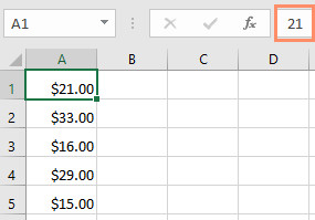
If you select any cell with a number format, you can see the cell's actual value in the formula bar. The spreadsheet will use this value for formulas and other calculations.

Excel 2016 - Lesson 8: How to format numbers in Excel (Number Formats) Picture 4

Use correct number format

There are more ways to format numbers than selecting cells and applying a format. Spreadsheets can actually apply a variety of number formats automatically based on how you enter the data. This means you'll need to enter the data in a way the program can understand and then ensure that the cells are using the appropriate number format.

For example, the image below shows how to use number formats for dates , percentages , and times :

Excel 2016 - Lesson 8: How to format numbers in Excel (Number Formats) Picture 5

Now that you know more about how number formats work, we'll take a look at some different number formats.

Percentage formats

One of the most useful number formats is the percentage format (%). It displays values ​​as percentages, such as 20% or 55%. This is especially useful when making calculations such as sales tax or interest. When you enter a percent sign (%) after a number, the percent number format is automatically applied to that cell.

Excel 2016 - Lesson 8: How to format numbers in Excel (Number Formats) Picture 6

In mathematical theory, a percent can also be written as a decimal. So 15% equals 0.15; 7.5% is 0.075; 20% is 0.20; 55% is 0.55 and more.

There are many times when percentage formatting is useful. For example, in the images below, note how the sales tax rate is formatted differently for each worksheet (5, 5% and 0.05):

Excel 2016 - Lesson 8: How to format numbers in Excel (Number Formats) Picture 7

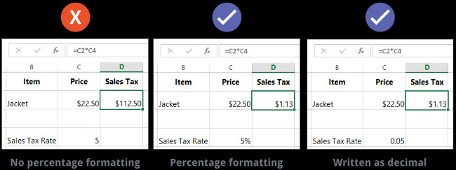
As you can see, the calculation in the spreadsheet on the left is not working correctly. Without the percentage format, the spreadsheet thinks we want to multiply $22.50 by 5, not 5%. And while the spreadsheet on the right still works without percentage formatting, the spreadsheet in the middle is easier to read.

Date formats

Whenever you work with dates, you'll want to use date formats to tell the spreadsheet you're referring to specific calendar dates, such as July 15, 2014. Date formats also allow You work with a set of date functions that use time and date information to calculate an answer.

Spreadsheets don't understand information the same way humans do. For example, if you enter October in a cell, the spreadsheet won't know you're entering a date so it treats it like any other text. Instead, when entering a date, you'll need to use a specific format that your spreadsheet understands, such as month/day/year (or day/month/year depending on the country you're in). In the example below, we'll enter 12/10/2014 as October 12, 2014. The spreadsheet will then automatically apply the date number format to that cell.

Excel 2016 - Lesson 8: How to format numbers in Excel (Number Formats) Picture 8

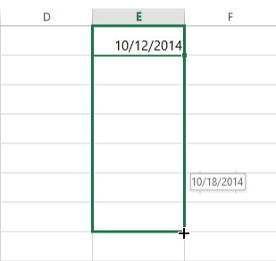
Now that we have a properly formatted date, we can do many other things with this data. For example, we could use a handle to continue the dates through the column, so a different date appears in each cell:

Excel 2016 - Lesson 8: How to format numbers in Excel (Number Formats) Picture 9

Excel 2016 - Lesson 8: How to format numbers in Excel (Number Formats) Picture 10

If the date format isn't applied automatically, it means the spreadsheet doesn't understand the data you entered. In the example below, we entered March 15. The spreadsheet doesn't understand we're referring to a date, so the cell is still using the general number format.

Excel 2016 - Lesson 8: How to format numbers in Excel (Number Formats) Picture 11

On the other hand, if we enter March 15 (without the "th"), the spreadsheet will recognize it as a date. Because it does not include the year, the spreadsheet will automatically add the current year, so the date will have all the necessary information. We can also enter the date in a number of other ways, such as 3/15; 3/15/2014 or July 15, 2014 and the spreadsheet will still recognize it as that date.

Try entering the dates below into the spreadsheet and see if the date formatting is applied automatically:

1. 12/10
2. October
3. October 12
4. October 2016
5. December 10, 2016
6. October 12, 2016
7. 2016
8. October 12

If you want to add the current date to a cell, you can use the keyboard shortcut Ctrl +; like in the video below:

More date format options

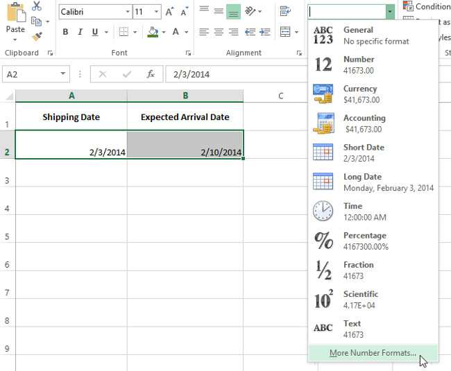
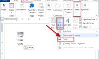
To access other date format options, select the Number Format drop-down menu and select More Number Formats . These are different date display options, like including the day of the week or omitting the year.

Excel 2016 - Lesson 8: How to format numbers in Excel (Number Formats) Picture 12

The Format Cells dialog box will appear. From here, you can select your desired date format option.

Excel 2016 - Lesson 8: How to format numbers in Excel (Number Formats) Picture 13

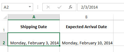
As you can see in the formula bar, custom date formatting doesn't change the actual date in the cell - it just changes how it's displayed.

Excel 2016 - Lesson 8: How to format numbers in Excel (Number Formats) Picture 14

Tips on number formatting

Here are some tips for getting the best results with number formatting:

Apply number formatting to entire columns : If you plan to use each column for a certain type of data, like dates or percentages, you may find it simplest to select the entire column by clicking the column letters and apply the number format you want. This way, any data you add to that column in the future will have the correct numeric format. Note that header rows will usually not be affected by number formatting.

Excel 2016 - Lesson 8: How to format numbers in Excel (Number Formats) Picture 15

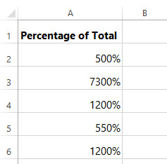
Recheck values ​​after applying number formatting : If you apply number formatting to existing data, you may have unexpected results. For example, applying percentage (%) formatting to a cell with a value of 5 will give you 500%, not 5%. In this case, you need to re-enter the value correctly in each cell.

Excel 2016 - Lesson 8: How to format numbers in Excel (Number Formats) Picture 16

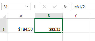
If you reference a cell with a number format in a formula, the spreadsheet can automatically apply the same number format to the new cell. For example, if you use a value with currency format in a formula, the calculated value will also use currency format.

Excel 2016 - Lesson 8: How to format numbers in Excel (Number Formats) Picture 17

If you want data to appear exactly as entered, you'll have to use text number formatting. This format is especially good for numbers that you don't want to perform calculations on, such as phone numbers, zip codes, or numbers that start with 0, like 02415. For best results, you can apply format text numbers before entering data into these cells.

Increase and decrease the number of digits after the comma

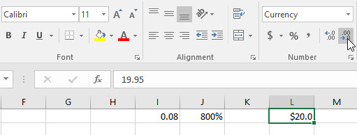
The Increase Decimal and Decrease Decimal commands allow you to control the decimal places displayed in a cell. These commands do not change the cell value; instead, they display values ​​for a set of decimal numbers.

Excel 2016 - Lesson 8: How to format numbers in Excel (Number Formats) Picture 18

Decrease Decimal will display the value rounded to that decimal place, but the actual value in the cell will still be displayed in the formula bar.

Excel 2016 - Lesson 8: How to format numbers in Excel (Number Formats) Picture 19

The Increase/Decrease Decimal command does not work with some number formats, such as Date and Fraction.

Refer to some more articles:

Next Excel lesson: Excel 2016 - Lesson 9: Working with multiple spreadsheets

Have fun!

Kareem Winters

Update 09 August 2024