Why Checkbox is an underutilized Excel feature?

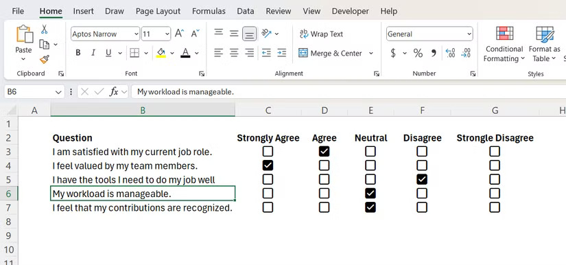
On the surface, Excel Checkboxes may seem like a very simple feature – which is probably why they are often overlooked. But when used properly, this often overlooked feature can turn your spreadsheets into interactive, user-friendly documents. Let's look at a few simple examples!

1. Create interactive surveys and forms

Excel Checkboxes provide a way to create interactive surveys and forms that mimic their online counterparts. This streamlines data collection, making them ideal for internal surveys, simple questionnaires, or collecting feedback.

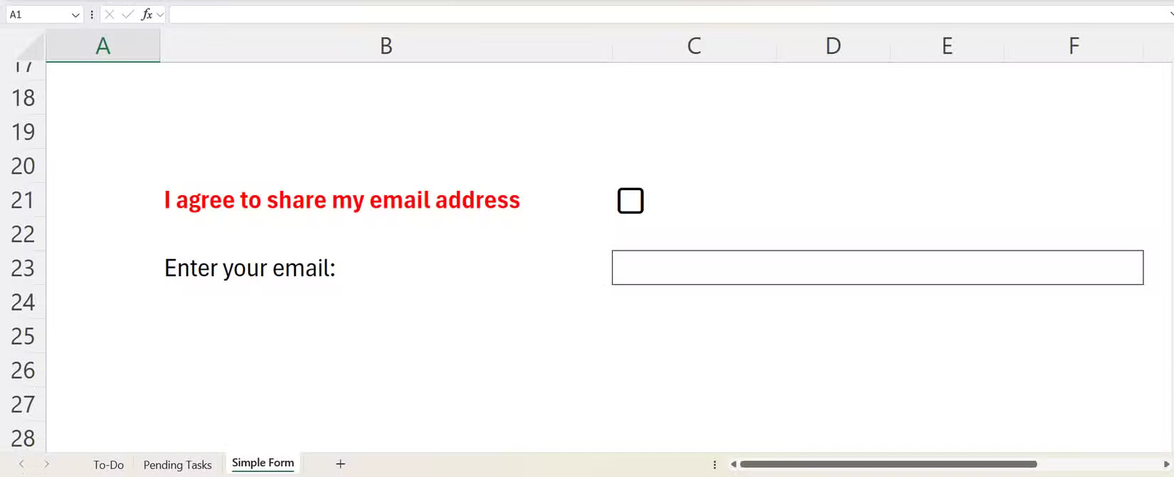
Checkboxes also allow for data validation. For example, you can ask users to agree to share their email addresses before entering them.

 

To do that, follow the steps below:

1. Click on the text box where the user must enter an email address.
2. Select the Data tab and click Data Validation in the Data Tools section of the ribbon.
3. In the Settings tab , click the drop-down menu below Allow and select Custom in the menu.
4. In the text box below Formula , type an equal sign followed by the cell containing the checkbox. In the example, the formula is =C21 .
5. Select the Error Alert tab .
6. In the text box below Error Message , enter the message you want to display if a user tries to enter their email address without checking the checkbox.
7. Click OK to close the dialog box and apply the changes.

If the user enters their email address without checking the checkbox, they will receive an error message.

2. Track tasks and important items

You don't need to download a separate app to create a to-do list. You can use Excel Checkboxes to track tasks, projects, inventory items, or attendees. For example, you can create a to-do list in an event planning spreadsheet with checkboxes to mark tasks as completed.

 

To take it a step further, you can use the FILTER function in Excel to filter out certain tasks based on whether they are checked or not. Create a new worksheet called Pending Tasks to filter out tasks that are not yet completed.

In a new worksheet, select the cell where you want to place the FILTER formula. The syntax should look like this:

=FILTER([array_range], [filter_range], [value_if_empty])

In the above example, both the array and the filter range are on the To-Do sheet . The array range is B4:B9 , where the task descriptions are, and the filter range is F4:F9 , where the checkboxes are. So the actual formula looks like this:

=FILTER('To-Do'!B4:B9,'To-Do'!F4:F9=FALSE, "")

Basically, this formula means that we want to display unchecked tasks as completed (equivalent to FALSE ). The double quotes at the end tell the formula to display nothing if there is no result. That way, you won't get an error message when the cell is blank.

Assuming everything is set up correctly, all uncompleted tasks will appear on the Pending Tasks sheet . Whenever you mark a task as complete on the To-Do sheet, it will disappear from the Pending Tasks sheet.

 

You can even create another sheet to track completed tasks. Just replace FALSE in the formula with TRUE and you're done.

3. Apply conditional formatting based on checkbox selection

Checkboxes also allow you to apply conditional formatting in Excel, making your spreadsheet more dynamic. For example, you can change the background color to green to make completed tasks easier to identify.

1. Select the range of cells you want to format.
2. In the Styles section of the Home tab , click Conditional Formatting > New Rule .
3. In the dialog box, select Use a formula to determine which cells to format .
4. Click inside the text below Format values ​​where this formula is true , then click the first checkbox. This will give you a formula that points to that checkbox.
5. Remove the second dollar sign from the formula. It will look like =$F4 .
6. Click the Format button .
7. Select the Fill tab , choose the color you want the formatted cell to change to, and click OK .

Tip : In Excel, the dollar sign ($) represents an absolute reference. When a formula has both absolute rows and columns, all formatting rules are applied to the first cell. This is why the second dollar sign must be removed.

Now, when you click the checkbox, Excel will automatically apply conditional formatting.

Checkboxes in Excel can do more than you think. While this article has covered some basic applications, you can explore more complex uses by combining checkboxes with other Excel functions and features. Experiment with them in your spreadsheets to unlock their full potential!