How to draw charts and graphs in Excel simply and quickly

Want to draw charts in Excel to present data vividly? Join Free Download to learn how to create common types of charts and editing tips for beautiful charts.

How to draw a chart in Excel

Note:  Instructions are performed on  Excel 2010 .

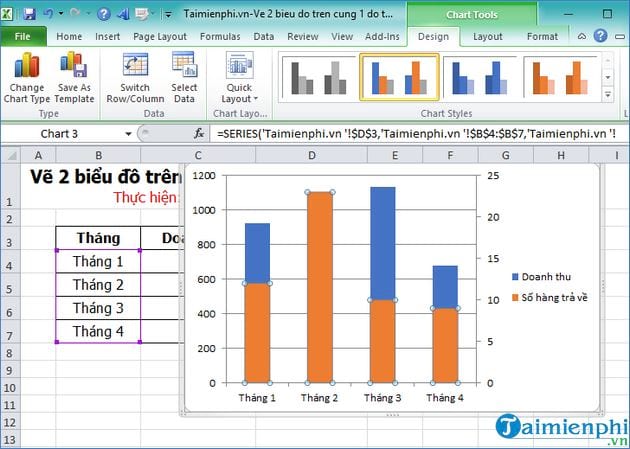
Suppose you have a data table as shown below and need to insert 2 charts on the same graph:

Step 1: Create a column chart

Select the data area, go to  Insert  => select  Column  => select  2-D Column .

Step 2: Transfer data to secondary axis

Click on the  Return Rows column.

Next, right click => select  Format Data Series

Step 3:  Select  Secondary Axis in Plot Series On .

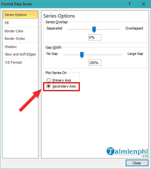
The result after you select  Secondary Axis  will be as shown below:

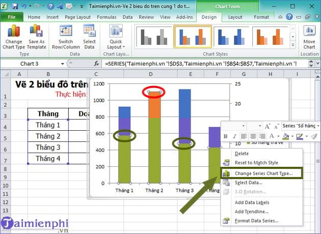
Step 4:  To draw a line chart for the  Returned Rows  column , do the following:

- Left-click on  Return row number  (at this time a circle will appear on all yellow columns).

- Next, right-click -> select  Change Series Chart Type

Then select  Line style  -> click  OK

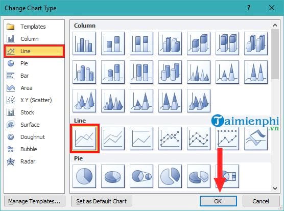
The result after you select is:

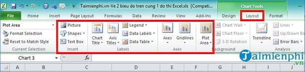
You can customize the chart to make it more beautiful. Go to  the Layout Tab  to add titles on the right, left, data on the columns. to make it reasonable and to your liking.

Excel provides many different types of charts such as bar, line, and pie charts to help present data visually. Users can customize colors, titles, and coordinate axes to make the chart more clearly displayed.

Additionally, if you need to plot multiple charts on the same worksheet, you can use the automatic sorting and alignment feature in Excel, which makes data management easier, especially when working with reports or analyzing data.