Instructions for coloring cells and text in Google Sheets

In Google Sheets supports you many ways to highlight cells in Google Sheets or cells with text in Sheets. We can use the cell coloring feature as usual in Sheets, or in the case of data filtering, we will use the conditional formatting setting for the data area that you want to color. The following article will show you how to highlight cells and text in Google Sheets.

How to highlight cells in Google Sheets with color

Step 1:

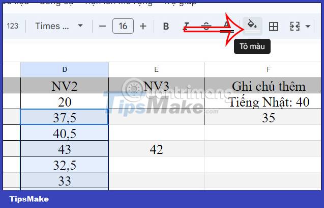
At the Excel table, the user first delineates the data that you want to color. Then we click on the paint bucket icon to choose to color.

Instructions for coloring cells and text in Google Sheets Picture 1

Step 2:

Now display the color palette interface for us to choose from. You click on the color you want to fill the selected data area.

Instructions for coloring cells and text in Google Sheets Picture 2

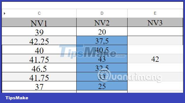
Then the data area has been colored as shown below.

Instructions for coloring cells and text in Google Sheets Picture 3

Instructions for alternating color in Google Sheets

In Google Sheets, there is an option to alternately color with the data area that the user wants, or alternately color the entire data table.

Step 1:

At the interface on Google Sheets, users click on Format and then select Alternate color in the displayed list.

Instructions for coloring cells and text in Google Sheets Picture 4

Step 2:

Displayed on the right edge of the screen you will see a selection of alternating colors. We will choose a Footer or Header color with a highlight box at the top or bottom.

Next click Apply to range to select the data area you want to select.

Instructions for coloring cells and text in Google Sheets Picture 5

Then you localize the data that we want to alternately color.

Instructions for coloring cells and text in Google Sheets Picture 6

Step 3:

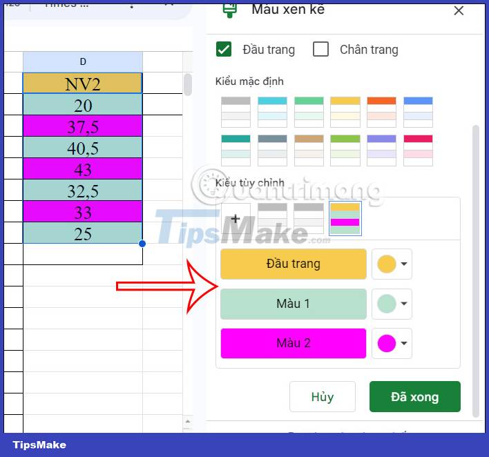
Now you choose the color you want to use for the selected data area.

Instructions for coloring cells and text in Google Sheets Picture 7

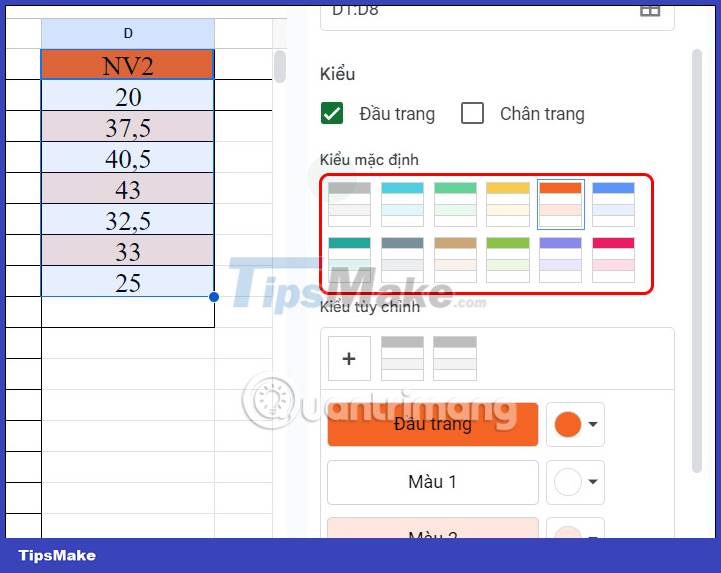
Or we can manually choose an alternative color for the alternate color we choose. After selecting the color, click Done to alternately color the data area.

Instructions for coloring cells and text in Google Sheets Picture 8

How to color in Google Sheets with conditional formatting

With this setting, you have a lot of different conditional formatting Google Sheets coloring options to color the data area.

Step 1:

Click on Format and then select Conditional Formatting displayed in the list below.

Instructions for coloring cells and text in Google Sheets Picture 9

Step 2:

On the right edge of the screen, the user chooses what condition you want to use at Format cells if… with a list of formats displayed as shown below. Then we choose the color to use.

Instructions for coloring cells and text in Google Sheets Picture 10

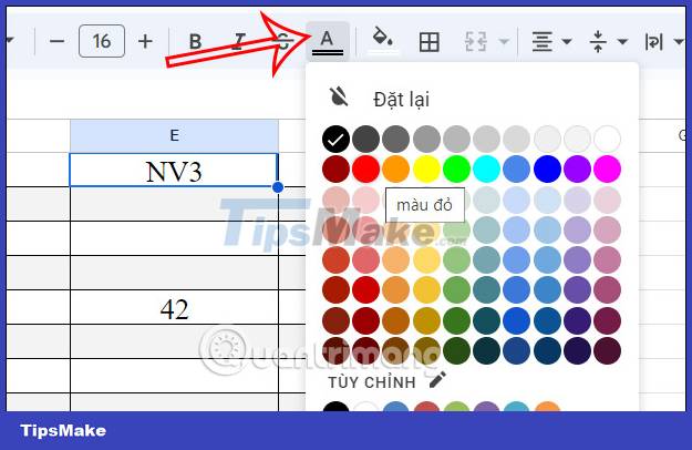
Instructions for coloring text in the Google Sheets box

To color only the text in the Google Sheets cell, users click on that cell , then click on the letter A icon to select the color you want to use for the text in this cell.

Instructions for coloring cells and text in Google Sheets Picture 11

Isabella Humphrey

Update 27 June 2023