How to use Name Box in Excel

You can go to anywhere in Microsoft Excel just by using this humble box. But where is the Name Box in Excel? It is located right next to the formula bar in a spreadsheet and displays the address of the selected cell or object. But that's just the most common usage. You can navigate around sheets with Name Box or use it as a powerful selection tool.

That's just a small part of the many things Name Box can do. Let's see all the functions that Name Box can bring you through the following article!

1. Find the address of the selected cell

How to use Name Box in Excel Picture 1

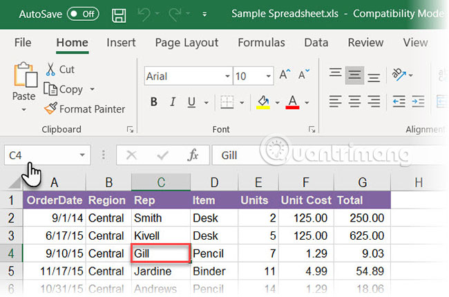
As shown in the screen above, the Name Box displays C4 because cell C4 is selected at the present time. Click on any cell to get its address and use it in the formula.

Name Box not only gives you the address of a cell. It can also be applied to any group of cells. For example:

1. Select a block : Name Box determines the first cell in the selected cell group.
2. Select a range of non-adjacent cells : You can select a number of cells that are not grouped together. Press Ctrl and select a series of non-adjacent cells. The Excel Name Box displays the address of the last cell you selected.

You can also go the other way. If you want to go to a specific cell or range of cells, you can enter the address of that cell in this Name Box and select them if needed.

Practice to see how the Name Box can help speed up your work, when you have multiple rows, columns and even sheets to handle.

2. Use the Name Box to select the box

Let your mouse rest! You can select a block with only their address.

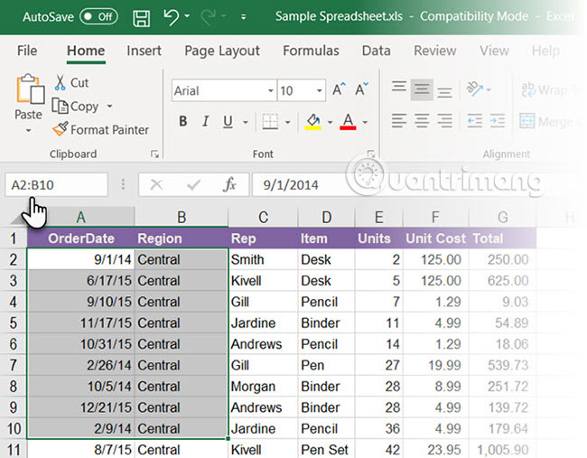
1. Select a block of cells : In the screenshot below, the author has typed A2: B10 into the Name Box and then press Enter . This will select a cell and you do not have to move on the worksheet with the mouse.

How to use Name Box in Excel Picture 2

1. Select a range of cells on another worksheet : Add a sheet reference (eg, Sheet2! A5: B10 ) in the Name Box.
2. Select multiple blocks : As shown in the example in the screen below, you can enter A1: A5, C1: C5, G1: G5 and then press Enter to select any number of non-adjacent cells. a time.

How to use Name Box in Excel Picture 3

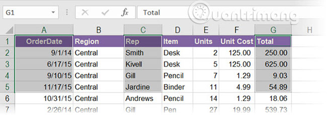
You can jump from any cell to another cell, just by entering these cell addresses. To move to any cell in another workbook that belongs to the same workbook, enter the worksheet name, an exclamation point, the cell address, and then press Enter . For example, Sheet2! A10.

3. Select rows and columns with Name Box

Use Excel's Name Box as another accelerator to quickly select rows and columns. These are handy Excel shortcuts when you want to avoid using the mouse.

1. Select the current row : Enter the letter R in Name Box and press Enter to select the current row.
2. Select the current column : Enter C in Name Box and press Enter to select the current column.

Remember that the letters R and C are Excel reserved for this reason and you cannot use these alphabets to create Named Ranges in Excel (learn more about Named Ranges below).

1. Select any number of rows : Suppose you want to highlight the first 5 rows, enter 1: 5 in Name Box and then press Enter to select rows 1 through 5. You must select two or more rows. If you enter a unique number into the Name Box (for example: 1 ) and press Enter , Excel displays an error message.

How to use Name Box in Excel Picture 4

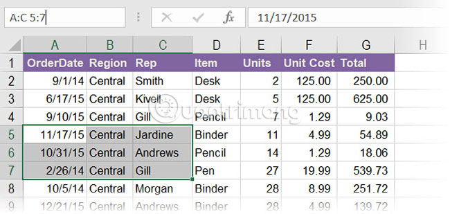
1. Select two or more columns : Suppose you want to highlight the first 5 columns, enter A: E in Name Box and then press Enter to select columns A through E. Again, you must select two or more columns.
2. Select specific rows and columns at the same time : You can even select multiple rows and columns at the same time. For example, type A: C, 5: 7 and press Enter to get the following selections.

This is very interesting because you can immediately see the values ​​of intersecting rows and columns. In the screen below, it is data in A5: C7 range .

How to use Name Box in Excel Picture 5

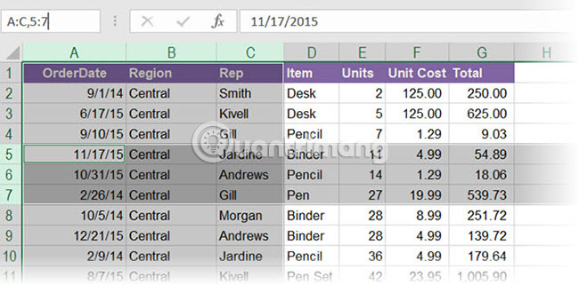
In the above case, you can also isolate the intersection between cells by entering A: C 5: 7 . Remove commas and include a space between the ranges to see that Excel highlights the cells where the two ranges intersect.

How to use Name Box in Excel Picture 6

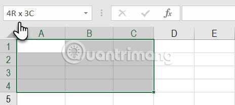
1. Find the total number of rows and columns : Name Box displays the total number of rows and columns when you click the left mouse button or hold the Shift key while selecting a block.

How to use Name Box in Excel Picture 7

4. Create Named Ranges for Excel formulas

Imagine an Excel spreadsheet that references some range of cells in many formulas. It's easy to be confused with alphanumeric cell names. If these cells have their own descriptive names, immediately tell you what these boxes are, wouldn't it be easier?

Excel uses the Named Ranges to do that. And you will use the Name Box in Excel to take advantage of this feature.

1. Step 1 : Select a cell or range of cells.
2. Step 2 : Name the description for the selection in the Name Box. Press the Enter key.
3. Step 3 : Use this name instead of the selected cell address or the address of the entire range in any recipe.

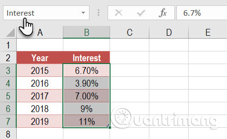
In the screen below, for example, assigned the Interest name to cells B3 to B7. Select the range that contains these cells, enter the word Interest in the Name Box, and then press Enter . All scope names in the workbook must start with a letter, underscore or backslash. Range names are not allowed with spaces.

How to use Name Box in Excel Picture 8

5. Name all objects in the Excel spreadsheet

A spreadsheet can have different objects such as images, charts, macro buttons, form control features such as buttons and checkboxes, etc. Excel uses common names like Chart 1, Chart 2 , . to name them. You can navigate through all objects by entering these names into the Name Box.

But like Named Ranges, making it easier to enter formulas, you can assign descriptive name objects to yourself, making it easier to find them.

How to use Name Box in Excel Picture 9

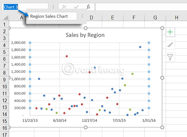
1. Step 1 : Select chart, image or object.
2. Step 2 : Place the cursor in Name Box and enter a new description name.
3. Step 3 : Press the Enter key.

6. Insert (or delete) multiple blank rows with Name Box

There are several ways to insert blank rows in Excel. One of them is with Name Box. This method is useful when you want to insert multiple rows at once. Go to Name Box and use the format of the starting row: ending row with numeric values ​​for the rows you want.

For example, if you want to insert 10 rows from row 2, enter 2:11 in the Name Box and press Enter . Excel will select the next 10 rows starting from row 2 (you must enter the number 11 because the second row will also count towards the next 10 rows).

How to use Name Box in Excel Picture 10

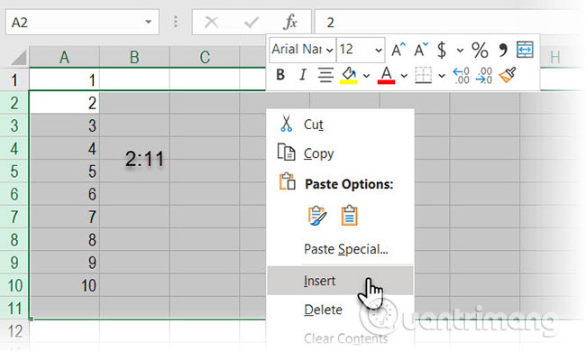
Then right-click on the selected row and select Insert. 10 empty rows will be inserted starting from row 2.

This method is useful when you want to insert thousands of empty rows for a number of reasons.

7. View Macro

How to use Name Box in Excel Picture 11

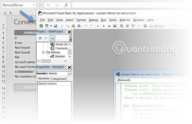
As mentioned before, you can name specific macro buttons in Excel. But you can also launch the Visual Basic editor to enter the source code for any macro.

Enter the name of the macro in Name Box. The VBA editor will open the macro source code for you to edit or view.

Using Name Box saves you a lot of time when working in Excel and that is why you should not ignore this utility. Because Name Box is a core navigation feature in Excel, you need to learn how to use it. Besides, creating Named Ranges and its ability to create quick selections shows how you can better capture a complex spreadsheet.

This is just one of many secret tools that save time and increase productivity when working in Excel.

Hope you are succesful.