How to use the AVERAGE function in Google Sheets

The AVERAGE function in Google Sheets has a similar use when you use the AVERAGE function in Excel, with the function formula being the same. AVERAGE function to calculate the arithmetic mean of a sequence of numbers, an array or reference containing numbers in the data table. Along with SUM function, AVERAGE function is one of the most basic Google Sheets functions when we process data tables. Using the function is very simple, users only need to determine the data area to be averaged. The following article will guide you how to use the AVERAGE function in Google Sheets.

1. How to count on multiple sheets of Google Sheets
2. How to link data between spreadsheets in Google Sheets
3. How to insert Google Sheets charts into Google Docs
4. How to set up the right to edit spreadsheets on Google Sheets

How to use the AVERAGE function in Google Sheets

AVERAGE function has the syntax to use = AVERAGE (number1, [number2], .) .

Inside:

1. number1: the first argument can be number, cell reference or range containing numbers to be averaged, required.
2. number2: are numbers, cell references or ranges containing additional numbers that want to calculate an average of up to 255 numbers, optional.

Note when using AVERAGE function:

1. The cell reference argument or range containing logical values, text or empty cells is automatically omitted, with the value 0 still being counted.
2. Logical values, indicating the number of text form entered directly into the list of arguments in the function will be counted.
3. If the argument is text or the value cannot be converted to a numeric error, an error occurs.

We will average students' test scores according to the data sheet below.

How to use the AVERAGE function in Google Sheets Picture 1

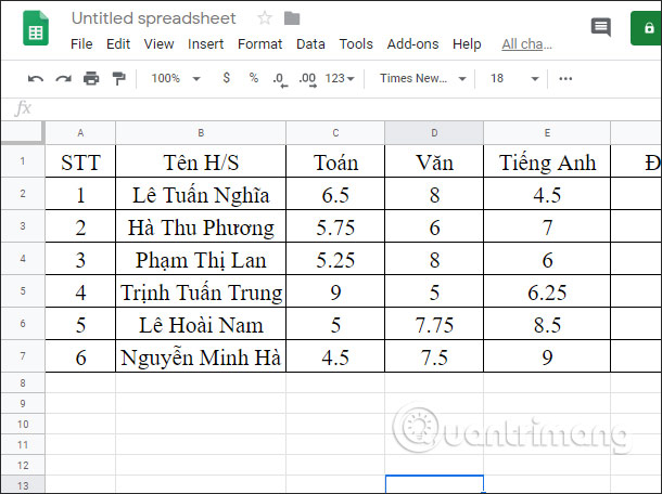
Step 1:

In the first point calculation box, enter the formula = AVERAGE (C2: E2) and press Enter.

How to use the AVERAGE function in Google Sheets Picture 2

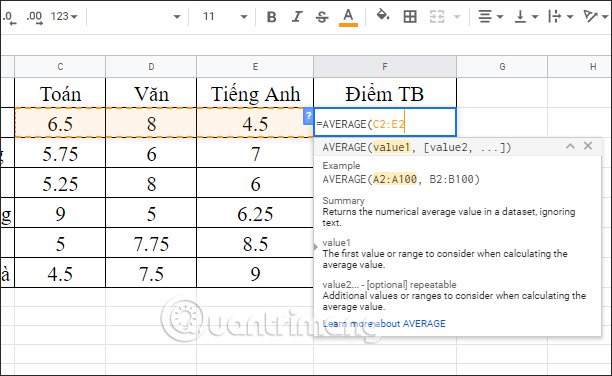
As a result we will see the average score of 3 subjects in the data table.

How to use the AVERAGE function in Google Sheets Picture 3

Step 2:

To calculate the average result for the remaining students, users just need to click on the first result box, then drag down the remaining cells.

How to use the AVERAGE function in Google Sheets Picture 4

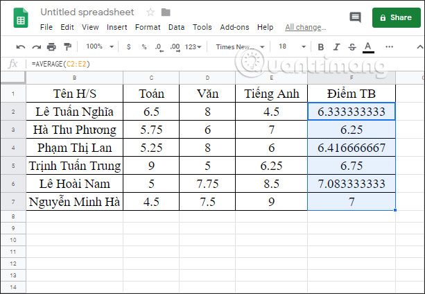
Step 3:

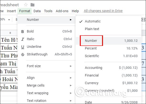
The resulting average spreadsheet displays the decimal number with many values ​​behind the period. To shorten the results , first black out the entire column and click on Format to edit the format.

How to use the AVERAGE function in Google Sheets Picture 5

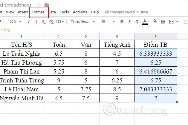
Step 4:

Next click on Number , then select Number format .

How to use the AVERAGE function in Google Sheets Picture 6

The average score of 3 subjects has been neatened as shown below.

How to use the AVERAGE function in Google Sheets Picture 7

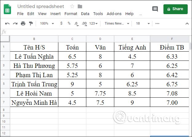
With the score of 0 behind you want to leave, just black out and then click on the 0 symbol with the left arrow to remove 0 . Each click is removed 1 after the decimal point.

How to use the AVERAGE function in Google Sheets Picture 8

So using the AVERAGE function in Google Sheets is very simple, there are not many combined data conditions. You only need to determine the area that needs to calculate the average of the total is okay.

I wish you all success!