How to rename, name rows or columns in Google Sheet

Named ranges, or named ranges, in Google Sheets allow you to add custom names to a group of cells in a worksheet, from entire columns or rows to smaller groups of cells. Creating a named range won't overwrite the original cell references (A1, A2, etc.), but it does make it easier to refer to these cells (and the data within them) as you create them. a new formula, calculation.

Use the namebox

The fastest way to add a named range to a Google Sheet is to use the name box. This is a small cell just to the left of the formula bar that shows you the cell reference of the currently selected (highlighted) cell in the worksheet.

To get started, open a sheet in Google Sheet and select a column or row that you want to rename. Then, replace the existing cell reference in the name box with a new name, and then press the Enter key to save your selection.

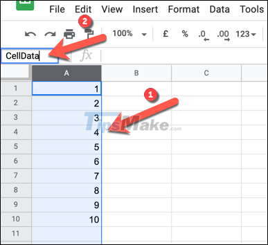
Google Sheet will immediately apply the new name to the column or row you selected. You can also view a list of available named ranges by clicking the down arrow button located to the right of the name box.

A list of named ranges, including their original cell references, will appear in the list below.

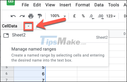
You can click on any named range to select those cells, or press 'Manage Named Ranges' to make changes to an existing naming range.

Using the named range menu

Another way to rename columns or rows is to use the naming range menu. This menu allows you to manage existing named ranges as well as create new ones.

Add a new named range

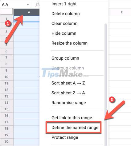
To get started, open a sheet in Google Sheet and select the column or row you want to rename. Next, right click on the selected cells and click 'Define The Named Range'.

Immediately, you will see a tabular menu titled "Named Ranges" Menu appear on the right side of the sheet. Enter your chosen name in the box provided. You can also change the selected column, row, or cell range to be smaller by changing the cell reference below it.

Press 'Done' to save your selection.

Edit or delete named ranges

To edit or delete a named range, right-click any cell in the spreadsheet and select 'Define The Named Range'.

You'll see a list of available named ranges in the sidebar on the right side of the window. Hover over the name in the 'Named Ranges' panel and press the 'Edit' button.

You can now make changes to the named range (including changing the name and the range of cells it refers to) using the available options. If you want to delete the named range, press the "Delete" button.

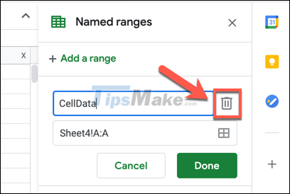
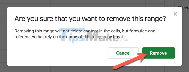
You will need to confirm your choice — press 'Remove' on the dialog box that appears afterwards.

Micah Soto

Update 24 June 2021