How to resize columns and rows in Google sheets

When you open a new spreadsheet on Google sheets, all the individual columns, rows, and cells you see on the screen will be of the same size. If you want more information, more data can be seen and displayed in each cell, you will need to change their size. Here's how to do it.

Manually resize columns or rows in Google Sheets

One of the fastest ways that you can use to resize columns or rows in Google Sheets is to manually order the mouse or trackpad. You just need to do simple operations like drag the column or row border to a new position until that column or row is expanded to the size you want.

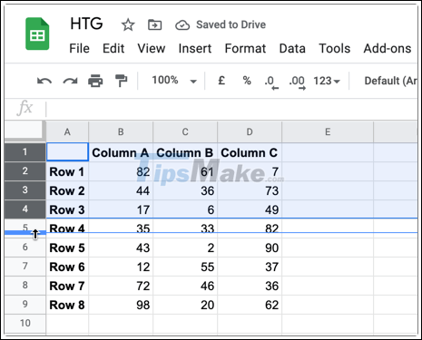
More specifically, first, open a Google Sheets spreadsheet containing the rows or columns that you want to resize. Below the formula bar you will see column headers, the default ranges from A to Z. Likewise, row headers are seen on the left side, default ranges from 1 to 100.

To resize a row or column, hover your mouse over the column heading (A, B, etc.) or row (1, 2, etc.) and hover over the border. Make sure your mouse pointer turns to an arrow icon, pointing in either direction.

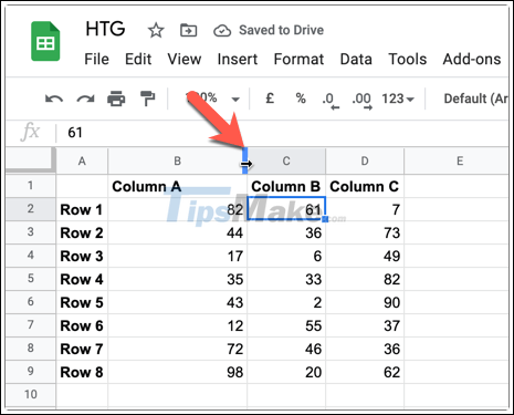
Use the mouse or trackpad to drag the border to a new position, and release only when the border is in the position you want. A blue line appears as the border is moving, giving you a visual indication of the new column or row size.

You can also complete this step for multiple columns or rows at once by highlighting them first, and then using the mouse or trackpad to resize the border on one of the columns or rows.

Google Sheets will automatically process selected cells together, changing all of them to a specific size.

Resize rows or columns automatically in Google Sheets

In Google Sheets, if cells in a row or column contain too much data, some information may be hidden, forcing you to click directly on the cell before it becomes fully viewable.

If you want to quickly resize these columns or rows to display the full data in the cell, you can use the mouse to resize automatically accordingly. This will reveal all hidden text, resize columns or rows to match the size of the largest cell, containing the most data.

First, open the spreadsheet and hover over the column headers (starting with A, B, etc.) or row (starting with 1, 2, and so on). Move the on-screen pointer over the border until the pointer changes to an arrowhead.

When the arrowhead pointer is displayed, double-click the border. This will force Google Sheets to automatically resize the corresponding row or column to fit the contents of the largest cell.

Similar to the manual method above, you can select multiple rows or columns to resize them at the same time. In general, this will automatically resize each row or column to fit the data of the largest cell.

Resize rows or columns in Google Sheets with the built-in tool

The above method allows you to flexibly resize columns and rows with mouse or touchpad. But if you want things to go faster and more accurate, use Google Sheets's built-in row and column resize tool.

First, open the worksheet that contains the row or column that you want to resize. Then click on the row's heading (starting with 1, 2, etc.) or column (starting with A, B, etc.) to select them.

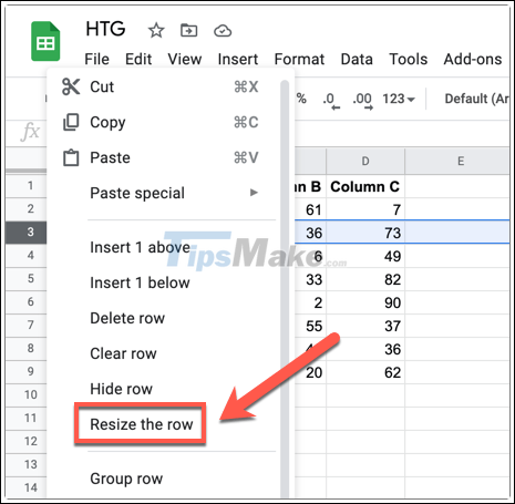
Right-click the title tag (for example, 1 or A). From the menu that pops up, click the ' Resize The Column ' or ' Resize The Row ' option respectively.

In the ' Resize ' dialog box for this row or column, enter a new dimension you want to apply to the row or column (the size in pixels). Also, check the option " Fit to data " to automatically resize the column or row to fit the data in the largest cell.

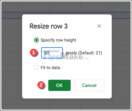
Click ' OK ' to make changes.

Immediately, the column or row will change to fit the size you selected. You can repeat this step for other rows or columns.

Kareem Winters

Update 25 February 2021