How to Highlight Every Other Row in Excel
This wikiHow teaches you how to highlight alternating rows in Microsoft Excel for Windows or macOS. Open the spreadsheet you want to edit in Excel. You can usually do this by double-clicking the file on your PC.
Table of Contents
Method 1 of 3:
Using Conditional Formatting on Windows
-
 Open the spreadsheet you want to edit in Excel. You can usually do this by double-clicking the file on your PC.
- This method is suitable for all types of data. You'll be able to edit your data as needed without affecting the formatting.
-
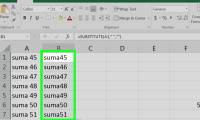
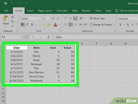 Select the cells you want to format. Click and drag the mouse so that all cells in the range you want to style are highlighted.[1]
- To highlight every other row of the entire document, click the Select All button, which is the gray square button/cell at the top-left corner of the sheet.
-
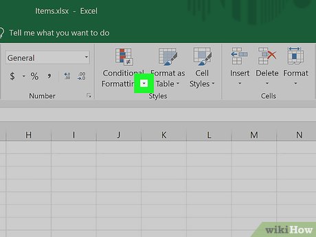 Click theicon next to "Conditional Formatting." It's on the Home tab in the toolbar that runs along the top of the screen. A menu will expand.
-
 Click New Rule. This opens the 'New Formatting Rule' dialog box.
 -
 Select Use a formula to determine which cells to format. You'll find this option under 'Select a Rule Type.'
- If you're using Excel 2003, set 'condition 1' to "Formula is."
-
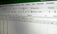
 Enter the formula to highlight alternating rows. Type the following formula into the typing area:[2]
- =MOD(ROW(),2)=0
-
 Click Format. It's a button on the dialog box.
 -
 Click the Fill tab. It's at the top of the dialog box.
 -
 Select a pattern or color for the shaded rows and click OK. You'll see a preview of the color below the formula.
 -
 Click OK. This highlights alternating rows in the spreadsheet with the color or pattern you selected.
- You can edit your formula or formatting by clicking the arrow next to Conditional Formatting (on the Home tab), selecting Manage Rules, and then selecting the rule.
Method 2 of 3:
Using Conditional Formatting on Mac
-
 Open the spreadsheet you want to edit in Excel. You can usually do this by double-clicking the file on your Mac.
 -
 Select the cells you want to format. Click and drag the mouse to select all the cells in the range you want to edit.
- If you want to highlight every other row in the entire document, press ⌘ Command+A on your keyboard. This will select all the cells in your spreadsheet.
-
 Click theicon next to "Conditional Formatting." You can find this button on the Home toolbar at the top of your spreadsheet. It will expand your formatting options.
-
 Click New Rule on the Conditional Formatting menu. This will open your formatting options in a new dialogue box, titled "New Formatting Rule."
 -
 Select Classic next to Style. Click the Style drop-down in the pop-up window, and select Classic at the bottom of the menu.
 -
 Select Use a formula to determine which cells to format under Style. Click the drop-down below the Style option, and select the Use a formula option to customize your formatting with a formula.
 -
 Enter the formula to highlight alternating rows. Click the formula field in the New Formatting Rule window, and type the following formula: [3]
- =MOD(ROW(),2)=0
-
 Click the drop-down next to Format with. This option is located below the formula field at the bottom. It will expand your formatting options on a drop-down.
- The formatting you select here will be applied to every other row in the selected area.
-
 Select a formatting option on the "Format with" drop-down. You can click an option here, and preview it on the right-hand side of the pop-up window.
- If you want to manually create a new highlight format with different color, click the custom format... option at the bottom. It will open a new window, and allow you to manually select fonts, borders and colors to use.
-
 Click OK. This will apply your custom formatting, and highlight every other row in the selected area on your spreadsheet.
- You can edit the rule at any time by clicking the arrow next to Conditional Formatting (on the Home tab), selecting Manage Rules, and then selecting the rule.
Method 3 of 3:
Using a Table Style
-
 Open the spreadsheet you want to edit in Excel. You can usually do this by double-clicking the file on your PC or Mac.
- Use this method if you want to add your data to an browsable table in addition to highlighting every other row.
- You should only use this method only if you won't need to edit the data in the table after applying the style.
-
 Select the cells you want to add to the table. Click and drag the mouse so that all cells in the range you want to style are highlighted.[4]
 -
 Click Format as Table. It's on the Home tab on the toolbar that runs along the top of the app.[5]
 -
 Select a table style. Scroll through the options in the Light, Medium, and Dark groups, then click the one you want to use.
 -
 Click OK. This applies the style to the selected data.
- You can edit the style of the table by selecting or deselecting preferences in the 'Table Style Options' panel on the toolbar. If you don't see this panel, click any cell in the table and it should appear.
- If you want to convert the table back to a regular range of cells so you can edit the data, click the table to bring up the table tools in the toolbar, click the Design tab, then click Convert to Range.
Was this article helpful?
Your feedback helps us improve.
Related Articles
 3 ways to highlight cells or rows in Excel7 minutes read
 How to use Focus Cell to highlight Excel data2 minutes read
 How to use Highlight in Word - Create and delete Highlight in Word?2 minutes read
 Steps to use Track Changes in Excel2 minutes read
 How to Remove Spaces Between Characters and Numbers in Excel3 minutes read
 5 real-world examples demonstrating the effectiveness of the MAP function in Excel.3 minutes read
Reader Comments 0
Sign in with email or Google to join the discussion.