How to hide and show the rows and columns in Excel is extremely simple.

In real work, there are times when you want to hide the rows or columns you don't want to show on the printout of an Excel spreadsheet. Or, after printing, you want to display the previously hidden rows and columns. This article will show you how to hide (Hide) and show (Unhide) column rows in Excel.

1. Hide (Hide) column rows in Excel

a. Hide rows in Excel

For example, you have a spreadsheet like this:

How to hide and show the rows and columns in Excel is extremely simple. Picture 1

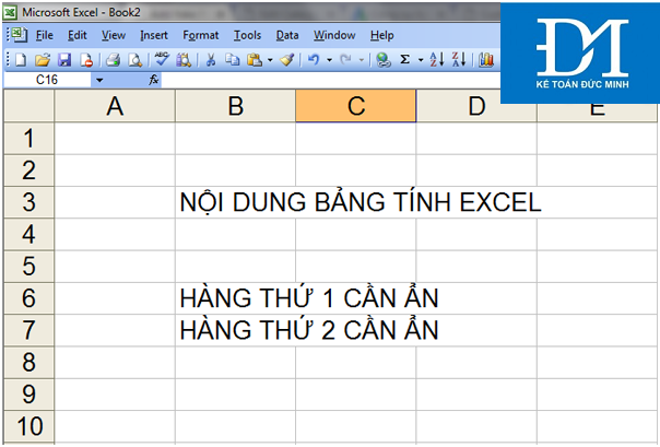
And you need to hide the 6th and 7th rows away.

+ Hide 1 row in Excel

In case you want to hide each row, you right-click on the row to hide (item 1) »Select Hide (item 2).

How to hide and show the rows and columns in Excel is extremely simple. Picture 2

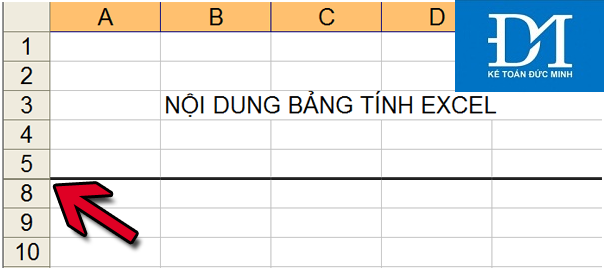
Once there, you will see the 6th row will be hidden as shown below:

How to hide and show the rows and columns in Excel is extremely simple. Picture 3

+ Hide multiple rows at once in Excel

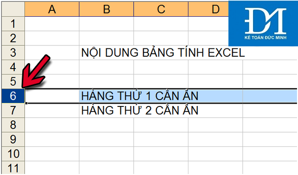
First, left-click and hold the left mouse button on the first row to hide in Excel worksheet:

How to hide and show the rows and columns in Excel is extremely simple. Picture 4

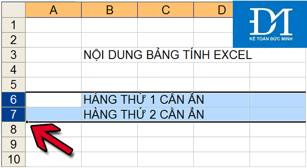
Next, you move the mouse down to select additional rows to hide. After selecting, release the left mouse button:

How to hide and show the rows and columns in Excel is extremely simple. Picture 5

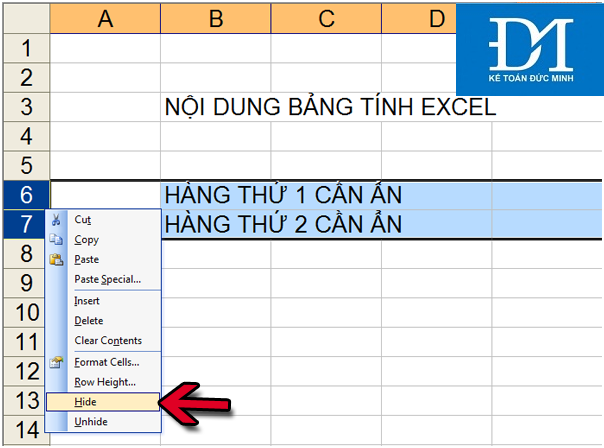
Right-click on the selected rows »Select Hide to hide those rows at the same time:

How to hide and show the rows and columns in Excel is extremely simple. Picture 6

Here is the worksheet after hiding 2 rows (Row 6 + 7):

How to hide and show the rows and columns in Excel is extremely simple. Picture 7

b. Hide columns in Excel spreadsheets

Suppose the table has 5 columns: No. (column A), Full name (column B), Age (column C), Occupation (column D), Interests (column E) as shown below:

How to hide and show the rows and columns in Excel is extremely simple. Picture 8

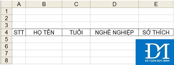
Now, you want to hide the Age column and the Interests column. We will do the following:

+ Hide 1 column in Excel

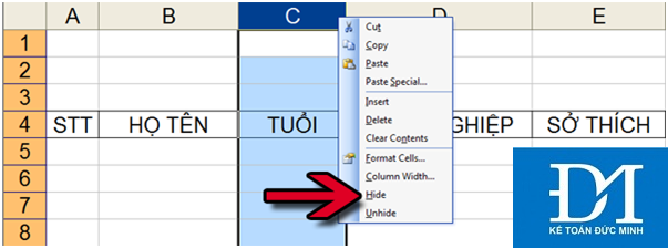
First, we will hide column C containing the Age column first by right-clicking on column C »Select Hide.

How to hide and show the rows and columns in Excel is extremely simple. Picture 9

And here is the result after hiding column C containing the Age column:

How to hide and show the rows and columns in Excel is extremely simple. Picture 10

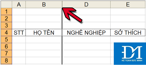
Do the same to hide the Occupation column (column D).

+ Hide multiple columns at once in Excel

First, left-click and hold the left mouse button on the first column to hide in the Excel spreadsheet. In this case, column C is the first column:

How to hide and show the rows and columns in Excel is extremely simple. Picture 11

Next, move your mouse to the right to select additional columns to hide. After selecting, release the left mouse button:

How to hide and show the rows and columns in Excel is extremely simple. Picture 12

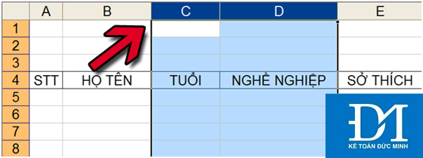
Next, right click on the selected area »Select Hide

How to hide and show the rows and columns in Excel is extremely simple. Picture 13

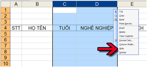
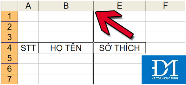
And here is the result after hiding the Age (column C) and Occupation (column D) columns at the same time:

How to hide and show the rows and columns in Excel is extremely simple. Picture 14

2. Display hidden column rows in Excel

a. Show hidden rows in Excel

Example of your original spreadsheet:

How to hide and show the rows and columns in Excel is extremely simple. Picture 15

After performing the operation hide 2 rows 6 and 7

How to hide and show the rows and columns in Excel is extremely simple. Picture 16

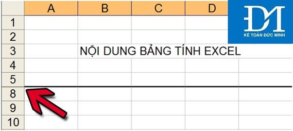
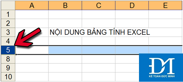
Now, if you want to display two hidden rows (row 6 and row 7), left-click on the first 5 rows:

How to hide and show the rows and columns in Excel is extremely simple. Picture 17

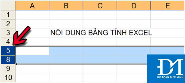
Then, move the mouse down to select additional row 8:

How to hide and show the rows and columns in Excel is extremely simple. Picture 18

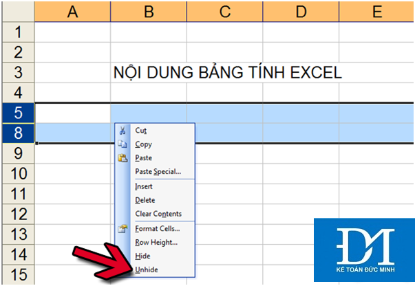
Right click on the selected area »Select Unhide:

How to hide and show the rows and columns in Excel is extremely simple. Picture 19

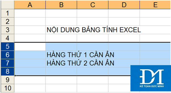
And the hidden rows are displayed:

How to hide and show the rows and columns in Excel is extremely simple. Picture 20

b. Show hidden columns in Excel

Initially we have the following Excel spreadsheet:

How to hide and show the rows and columns in Excel is extremely simple. Picture 21

After hiding the Age column (column C) and Occupation column (column D), the remaining worksheet:

How to hide and show the rows and columns in Excel is extremely simple. Picture 22

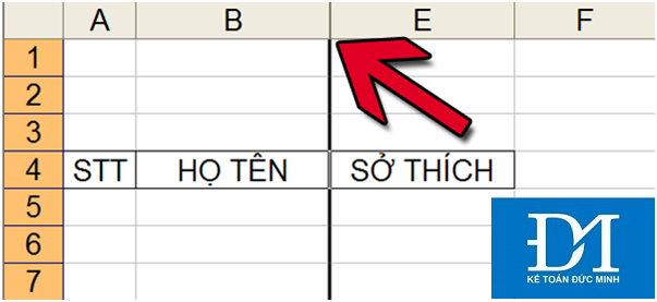
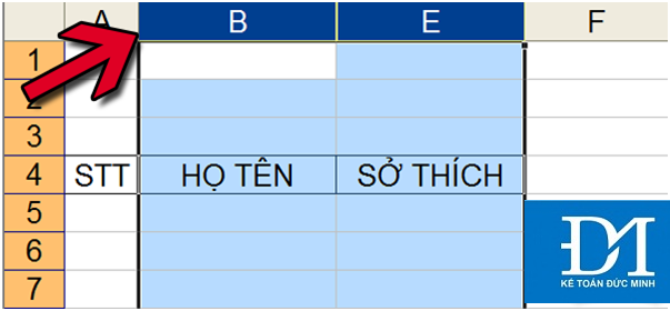
Now, we will show the hidden columns C and D again by holding down the left mouse button on column B, then moving the mouse to the right to select additional column E. Then release the left mouse button:

How to hide and show the rows and columns in Excel is extremely simple. Picture 23

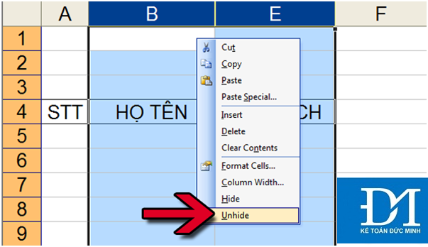
Right click on selected area »Select Unhide:

How to hide and show the rows and columns in Excel is extremely simple. Picture 24

And this is the result:

How to hide and show the rows and columns in Excel is extremely simple. Picture 25