How to freeze, hide rows and columns in Google Sheets

When working with Google Sheets, you will have to handle dozens of data columns. And if you're mistakenly dealing with multiple columns, you can freeze unused columns, or hide columns or rows to make Google Sheets more compact.

Columns or rows that have been frozen or hidden will not be visible or clickable to operate. If the title row is frozen, the document is easier to read. Besides, column freezing also has many different options, besides freezing the first row or column. The following article will guide you how to freeze, hide rows and columns in Google Sheets.

1. Tips to use Google Sheets should not be overlooked
2. How to edit chart notes in Google Sheets
3. How to add or delete rows and columns in Google Sheets
4. How to link data between spreadsheets in Google Sheets

1. Freeze columns and rows of Google Sheets

Step 1:

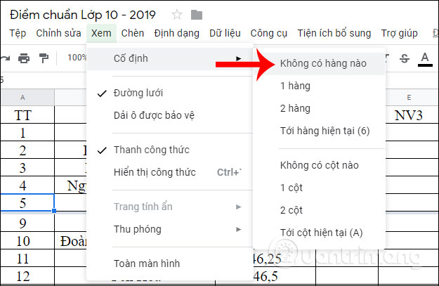
You click on the row or column you want to freeze, then click on the View select Fixed .

How to freeze, hide rows and columns in Google Sheets Picture 1

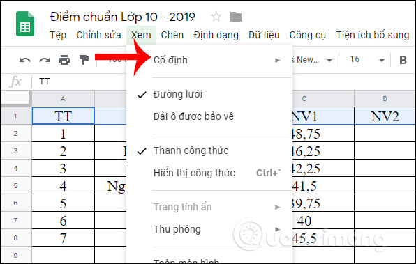
Now show more options to fix columns and rows. If you press 1 row or 1 column, the first row and column selected are closed. If you press 2, the first 2 rows and 2 columns are frozen.

How to freeze, hide rows and columns in Google Sheets Picture 2

Step 2:

The result of the row or column you selected has been frozen. They are fixed by a gray border to separate them from the area, and cannot be moved no matter where you drag the mouse to any position.

How to freeze, hide rows and columns in Google Sheets Picture 3

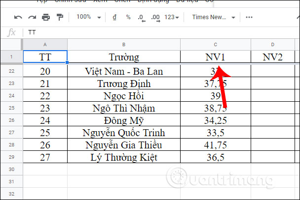
If the user wants to freeze the entire row or column , first click the mouse in the last cell in the row or column to be frozen. Google Sheets will count from the first row and column down to the position where you clicked. Then click View, select Fixed, then select Go to current row / column .

How to freeze, hide rows and columns in Google Sheets Picture 4

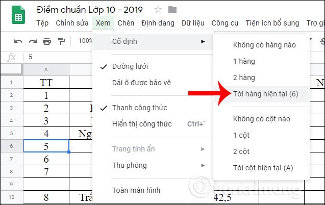
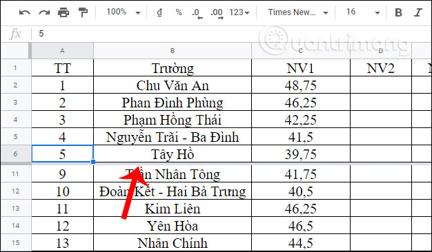
For example, I will freeze from the first row to the 6th row, then click in cell 5. Now Google Sheets counts there are 6 rows that need to be frozen.

The first 6 rows of results have been fixed.

How to freeze, hide rows and columns in Google Sheets Picture 5

Step 3:

If you want to unfreeze the column or row, click on View, select Fixed and then select K without any rows (columns) .

How to freeze, hide rows and columns in Google Sheets Picture 6

2. Hide columns and rows in Google Sheets

Step 1:

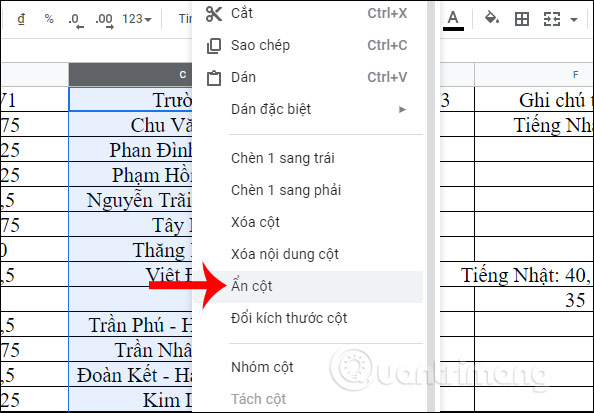
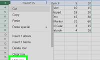
First, click the column header at the top and right-click and choose Hide column .

How to freeze, hide rows and columns in Google Sheets Picture 7

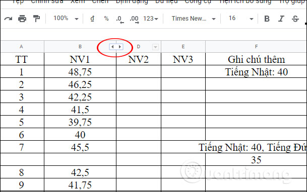
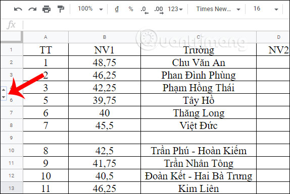
The selected column is now hidden and is indicated by two arrows on either side of the hidden column. If you click this arrow icon , the column will automatically display .

How to freeze, hide rows and columns in Google Sheets Picture 8

Step 2:

To hide rows in Google Sheets, users do the same, click on the first row of the row and select Hide rows .

How to freeze, hide rows and columns in Google Sheets Picture 9

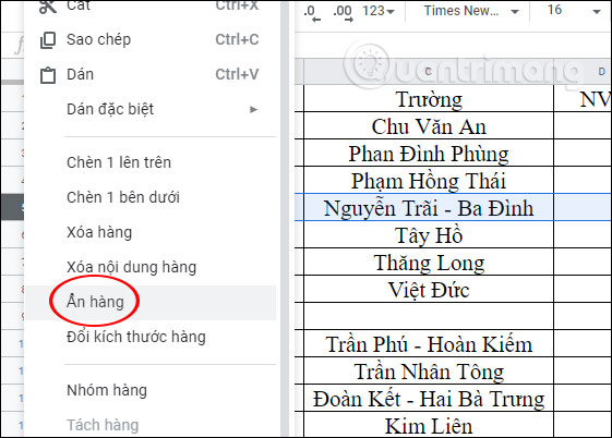
The result of the row has been hidden and an arrow icon appears to indicate that a row has been hidden. To display the row again, just click the arrow icon.

How to freeze, hide rows and columns in Google Sheets Picture 10

Manipulating rows, columns and hiding rows and columns in Google Sheets is simple and easy to follow. When done, users cannot operate on locked or hidden areas, making it easier to tidy up the data table.

I wish you successful implementation!