How to Hide Rows in Excel

Method 1 of 2:

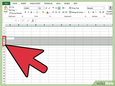Use the row selector to highlight the rows you wish to hide. You can hold the Ctrl key to select multiple rows.
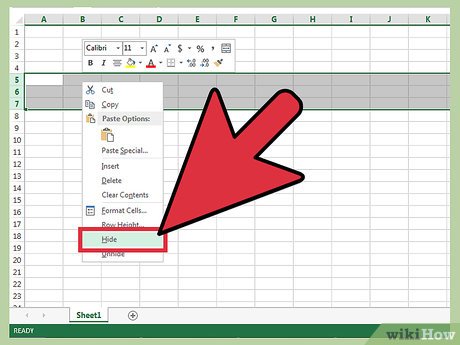Right-click within the highlighted area. Select 'Hide'. The rows will be hidden from the spreadsheet.
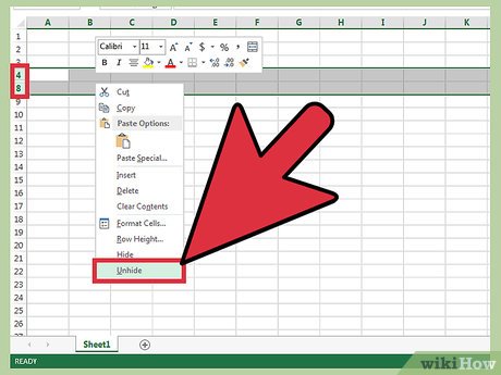Unhide the rows. To unhide the rows, use the row selector to highlight the rows above and below the hidden rows. For example, select Row 4 and Row 8 if Rows 5-7 are hidden.
1. Right-click within the highlighted area.
2. Select 'Unhide'.

Method 2 of 2:

Create a group of rows. With Excel 2013, you can group/ungroup rows so that you can easily hide and unhide them.
1. Highlight the rows you want to group together and click "Data" tab.
2. Click "Group" button in the "Outline" Group.
Hide the group. A line and a box with a (-) minus sign appears next to those rows. Click the box to hide the "grouped" rows. Once the rows are hidden the small box will display a (+) plus sign.
Unhide the rows. Click (+) box if you want to unhide the rows.

Jessica Tanner

Update 05 March 2020

You should read it