The easiest way to Hide rows in Excel

Select and hide multiple rows

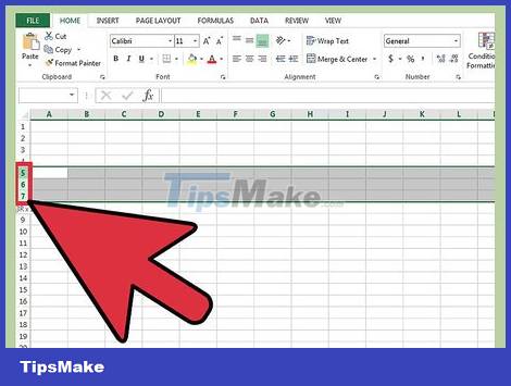
Use the selection cursor to highlight the rows that you want to hide. You can hold down the Ctrl key to select multiple rows.

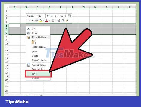
Right click on the highlighted area. Select 'Hide'. The selected rows are hidden from the sheet.

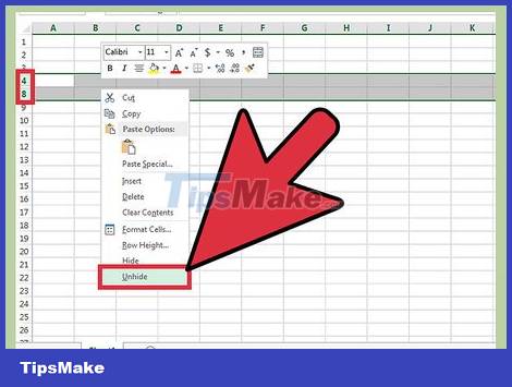
Unhide the rows. To do this, use the selection cursor to highlight the rows above and below the hidden row. For example, you would select row 4 and row 8 if rows 5-7 are hidden.

Right click on the highlighted area.

Select 'Unhide'.

Hide merged rows

Consolidate goods. With Excel 2013, you can merge/unmerge rows to easily hide and unhide them.

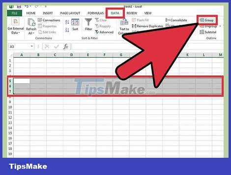
Highlight the rows you want to merge and click the "Data" tab.

Click the "Group" option in the "Outline" option group.

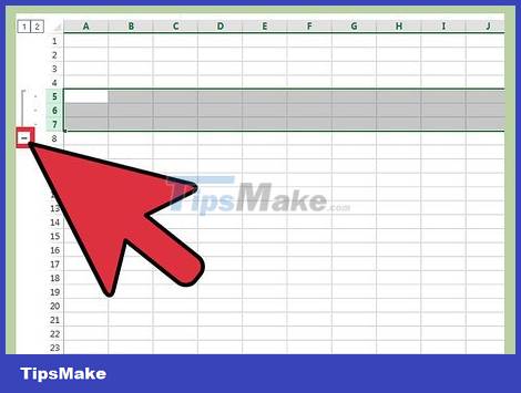
Hide merged rows. You should see a line and a box with a minus sign (-) inside appear next to the merged rows. Click the box to hide the merged rows. Once hidden, a plus sign (+) will be displayed in the box.

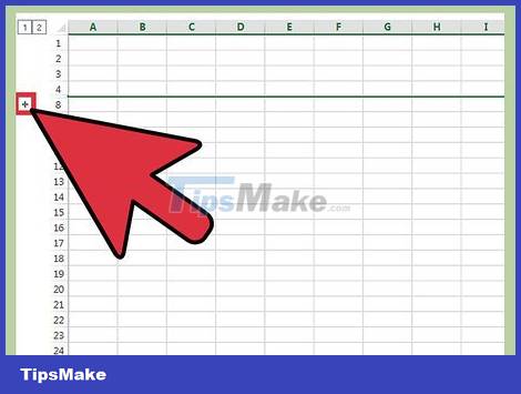
Unhide merged rows. If you want to unhide these rows, just click in the box with the plus sign (+).