Change Color Between Different Lines in Microsoft Excel

Change Color Between Different Lines in Microsoft Excel covers the essential facts behind the topic, including what changed, why it mattered, and how it affected users.

Instructions Overview

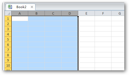
First, open Excel and select the data area to fill, or press Ctrl + A to select all:

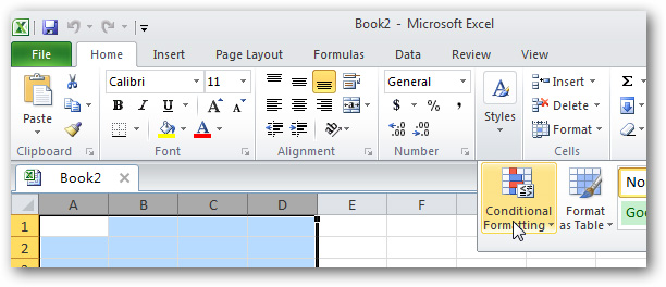
Select the Home tab above and Styles> Conditional Formatting:

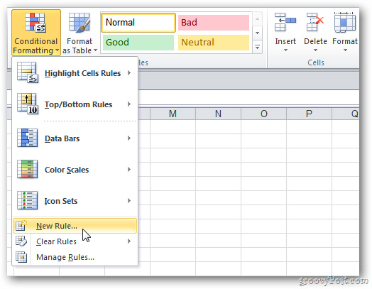
Menu with the form of drop - down displayed, you select New Rule:

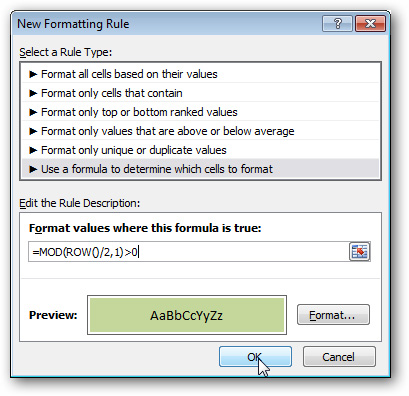
The New Formatting Rule window is displayed, click the button at the bottom of the screen with the name: Use a Formula to Determine Which Cells to Format. If the data field is empty, you use the following formula:

= MOD (ROW () / 2.1)> 0

The New Formatting Rule window will look like this:

Click the Format button, then select the color to use, click OK:

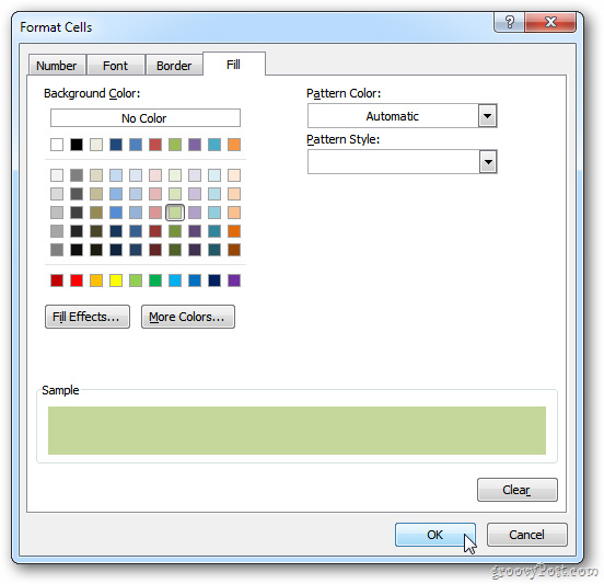
Color preview - Color Preview displays on the New Formatting Rule window as shown below, click OK:

And the data on your spreadsheet will be colorized based on the value and applicable rules. Example as shown below:

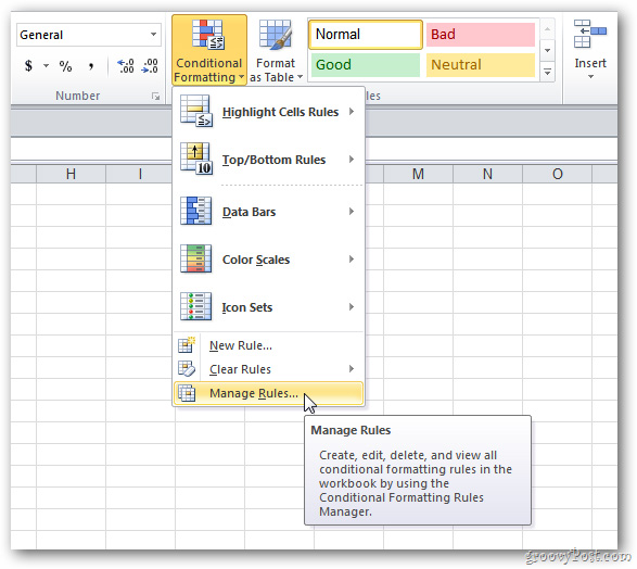
If you want to change the color or add or remove the data stream, we just need to select the corresponding cell, then select Conditional Formatting> Manage Rules:

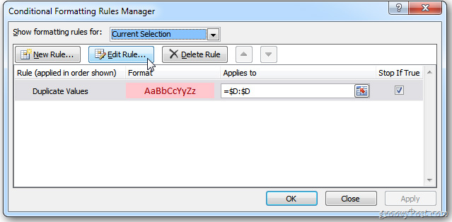
The Conditional Formatting Rules Manager window appears, click the Edit Rule button:

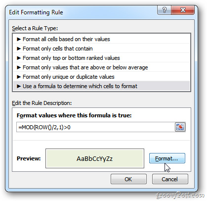
We will be returned to the Edit Formatting Screen section, here you can adjust and set the conditions to change at will:

Good luck!

>>> Video guide for reference: