How to Calculate Quartiles in Excel

Using "QUARTILE.INC"

1. 
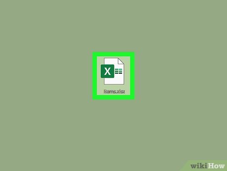
   Open your project in Excel. If you're in Excel, you can go to File > Open or you can right-click the file in your file browser.

   1. This method works for Excel for Microsoft 365, Excel for Microsoft 365 for Mac, Excel for the web, Excel 2019-2007, Excel 2019-2011 for Mac, and Excel Starter 2010.
2. 
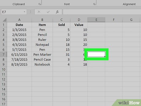
   Select an empty cell where you want to display your quartile information. This can be anywhere on your spreadsheet.

   1. For example, you can select cell E7 even if all your data is located in cells A2-A20.
3. 
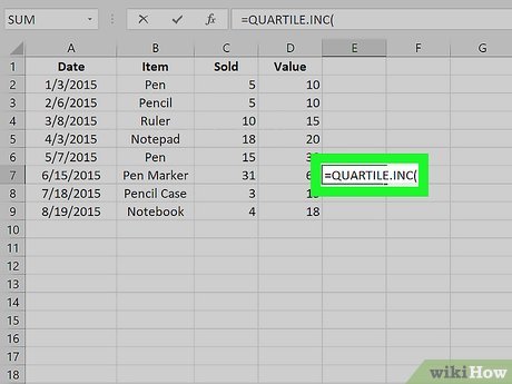   Enter the quartile function: =QUARTILE.INC(. INC stands for "Inclusive," which will give you results that include 0+100.
4. 
   Select the cells containing your data. You can drag your cursor to select the entire range or you can select the first cell then press CTRL + SHIFT + Down arrow.

   1. After you've selected the data set, you'll see it entered into your formula. It'll look something like "=QUARTILE.INC(A2:A20". Don't add the closing parentheses because you'll need to add more information to the function.
5. 
   Enter ",1)" to finish the formula. The number after the data range can represent either Q1, Q2, Q3, or Q4, so you can use any number 1-4 in the function instead of 1.

   1. The function QUARTILE.INC(A2:A20,1) will show you the first quartile (or 25th percentile) of your data set.^[1]
6. 
   Press ↵ Enter (Windows) or ⏎ Return (Mac). The cell you have selected will display the quartile function result. You can repeat this process using the other quartile function to see the differences.^[2]