How to Use the FIND Function in Excel?

This guide explains how to use FIND Function in Excel, including its syntax, required arguments, practical examples, and common errors.

Instructions for using the FIND function in Excel

The syntax of the FIND function: = FIND (find_text; within_text; [start_num]) .

Inside:

• find_text: a character or text to search for a location.
• within_text: the text in which you want to find find_text.
• [start_num]: specify the start search position within within_text.

Note when using the FIND function:

• The FIND function is case-sensitive and in-text, while Excel SEARCH function is not case-sensitive.
• The FIND function does not support searching for characters like * find_text, find_text *, * find_text *.
• Use [start_num] to skip the first number of characters and start at the specified position, if omitting [start_num], the default will be = 1.
• If start_num is less than 0 or greater than the length of within_text, the function returns the error value.

1. FIND function example in Excel

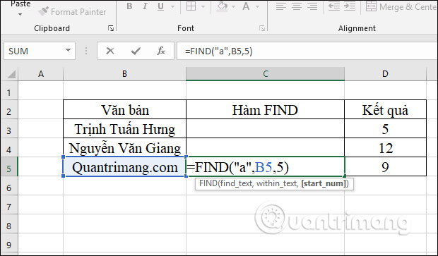
1. Find the position of the letter 'h' in cell B3 and have the function perform = FIND ('h', B3) and press Enter. The result will be 5 because the first 'h' is at the 5th position in the text string, distinct from the 'H'.

2. Find the position of the word 'Giang' in cell B4, so use to find_text = Giang to find the position. Function used with the command = FIND ('Giang', B4). The result returns the first character position of the word 'Giang' in the text. If there is no 'Giang' in the text string, the #VALUES!.

3. Find the position of the letter 'a' in the text string starting with the 5th character . For this example, you will need to use start_num as 5. The function has the formula = = FIND ('a', B5,5) and the result is 9 for the position of the character 'a' in the text string, adjectives character 5.

2. The FIND function example combines the LEFT function

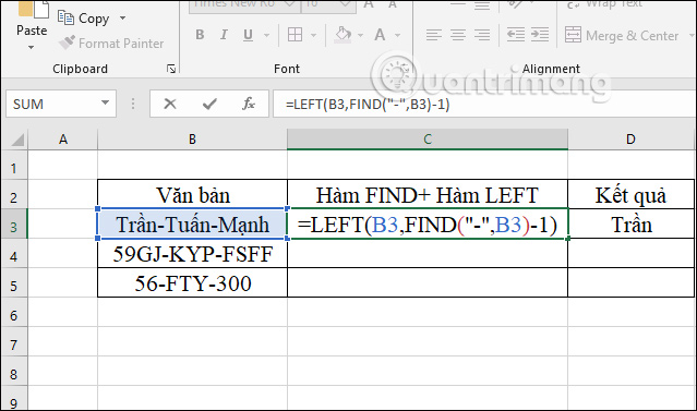
The FIND function in combination with the LEFT function is used to separate the first character string as in the first name, last name, area code, symbol, etc.

Finds the first character in cell B3 from left to right until it meets the character '-' and doesn't take the character '-' so there will be -1 in the function formula. We will have the combined function formula is = LEFT (B3, FIND ("-", B3) -1) and the result is Tran.

3. The FIND function example combines the MID function

When combining these two functions, we will find the middle character in the text string.

Find the first '-' character in cell B4 with the FIND function, then use the MID function to separate the two characters before and after the '-' character in the text string, resulting in the middle character. The function to use is = MID (B4, FIND ("-", B4) +1, 3) and then press Enter. The result is KYP characters.

4. Error correction of the #VALUE! Function in FIND

Report error #VALUE! in FIND function can be caused by 2 common errors.

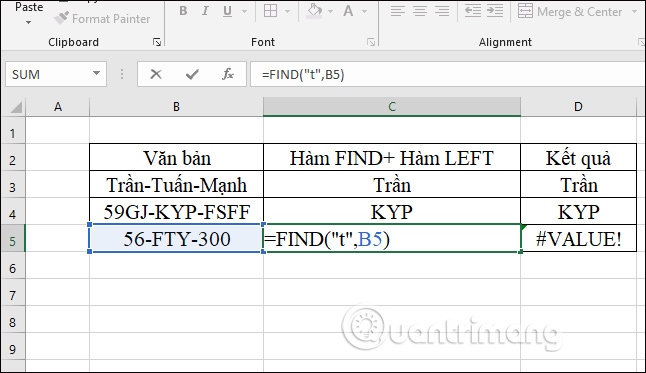
Cause 1 : The reference value could not be found in the text string.

For example, the following formula for the FIND function reports an error because the FIND function is case sensitive. So in B5 are all uppercase letters that lowercase search function will error. Or, if there is no character to look for in the text string, also #VALUE!.

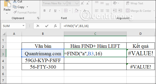
Cause 2 : Error [start_num] exceeds characters in the range

For example, finding the character 'a' in any position from character 16 will give an error because the text string has all 15 characters. Now you need to correct [start_num] properly.