Hide and show chart labels in Excel

The following article gives you detailed instructions on how to show / hide chart labels in Excel 2013.

Hide and show chart labels in Excel Picture 1

For example, the following chart has been created:

Hide and show chart labels in Excel Picture 2

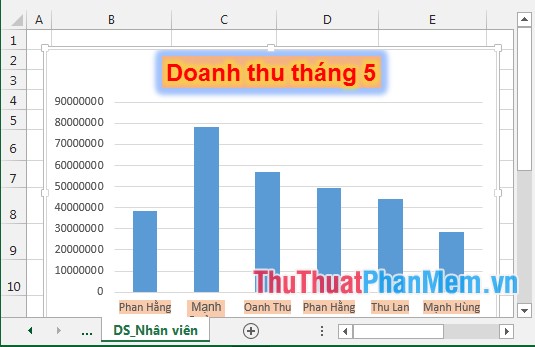
1. Want to add detailed sales for employees displayed right on the chart do the following:

- Click on the chart -> Design -> Add Chart Element -> Data labels -> select the data placement, for example, choose OutSide End :

Hide and show chart labels in Excel Picture 3

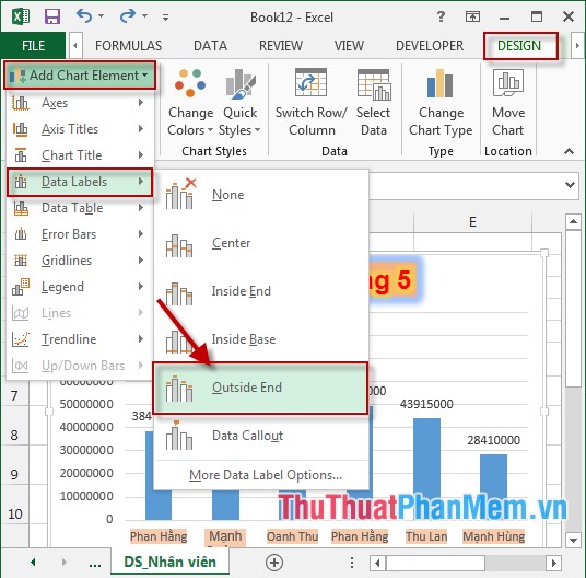
- Revenue data results show after the end of the data column:

2. Show more Legend tags.

2.1 Display of the Legend label.

- Click on the chart -> Design -> Add Chart Element -> Legend -> choose a label location, for example choose Top:

Hide and show chart labels in Excel Picture 4

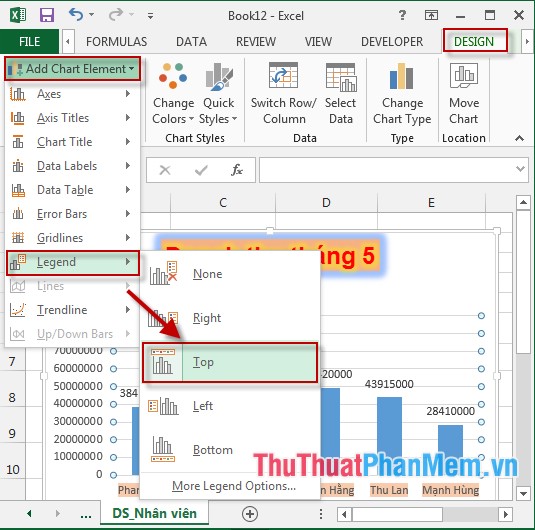
- The label results showing the chart content are displayed:

Hide and show chart labels in Excel Picture 5

2.2 Edit the labels.

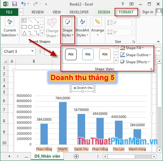
To edit the label -> click on the label name, for example, here edit the revenue label .

Step 1: Click on the label to edit -> Format -> Shape Styles -> select the features to adjust the frame of the label:

+ Shape Fill: Fill the background for the label frame.

+ Shape OutLine: Paint the border for the frame of the label.

+ Shape Effects: Create effects for frames of labels.

Hide and show chart labels in Excel Picture 6

Step 2: Edit the text content in the label:

Click on the label to edit -> Format -> WordArt Styles -> select the following format styles:

+ Text Fill: Coloring text.

+ Text Outline: Coloring borders for text.

+ Text Effects: Create effects for text.

Hide and show chart labels in Excel Picture 7

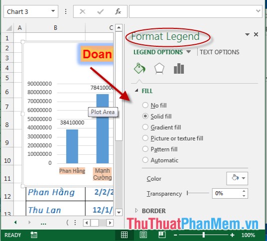
- In addition to the above, double-click the label name -> Format Legend dialog box displayed -> customize the properties for the label in this dialog box:

Hide and show chart labels in Excel Picture 8

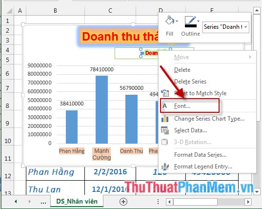
Step 3: Change the font, font size for labels. If you think the label is a bit small or want to change the font, do the following:

- Right-click on the label -> Select Font:

Hide and show chart labels in Excel Picture 9

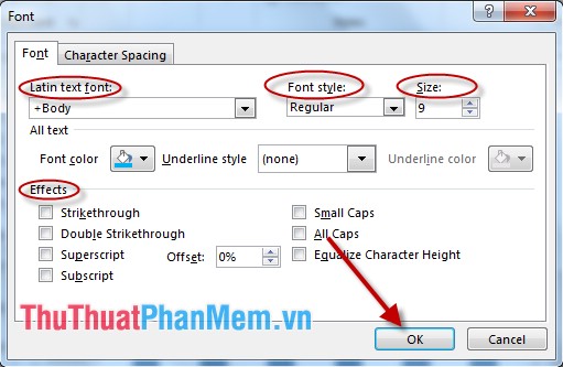
- The Font dialog box appears -> change the options for labels in the dialog box -> finally click OK to finish.

Hide and show chart labels in Excel Picture 10

- After performing the above steps, the results are:

Hide and show chart labels in Excel Picture 11

- If you do not want to display the Legend, click on the chart -> Design -> Add Chart Element -> Legend -> None the label is automatically removed on the chart:

Hide and show chart labels in Excel Picture 12

The above is a detailed guide on how to hide / show chart labels in Excel 2013.

Good luck!

4 ★ | 1 Vote

May be interested

  • Steps to reset chart in ExcelSteps to reset chart in Excel
    the following article shows you the steps to reset the chart in excel 2013. after creating the chart, if you do not like the selected chart style, you can do the following to change the chart type the simplest and fastest way: step 1: sign
  • How to fix chart position in ExcelHow to fix chart position in Excel
    when you position the chart in excel, users can easily change the size of the column in the worksheet without affecting the position and size of the chart.
  • How to hide, show notes in tables on ExcelHow to hide, show notes in tables on Excel
    the feature of commenting and commenting on excel data sheet will help viewers better understand, more detailed information about the content in the row or column.
  • How to make a thermometer template in ExcelHow to make a thermometer template in Excel
    using a thermometer chart in excel is a good choice for keeping track of financial goals. here are detailed step-by-step instructions on how to make a heat chart in excel.
  • How to hide and show Sheet in ExcelHow to hide and show Sheet in Excel
    sometimes working with too many sheets makes you confused, or you don't want important sheets being viewed by others on your computer ..., or for some reason you want to hide the sheet and when necessary then display the sheet.
  • How to create 2 Excel charts on the same imageHow to create 2 Excel charts on the same image
    the combination of 2 charts on the same excel image helps users easily show the data.
  • 'Moving' chart in Excel'Moving' chart in Excel
    do you see a motion chart in excel? with a simple, self-created viual basic program, you can make your chart move to look lively. suppose, you have a data table with column a containing the variable x (from a4: a19).
  • How to Create a Bar Chart in ExcelHow to Create a Bar Chart in Excel
    wikihow will show you how to present data in microsoft excel more eye-catching and attractive with bar charts.
  • Types of data hiding in Excel - Part end: Hide Excel FilesTypes of data hiding in Excel - Part end: Hide Excel Files
    today tipsmake will show you the last part: 'hide excel file' in the series 'guide all types of hidden data in excel extremely useful'.
  • How to hide formulas in ExcelHow to hide formulas in Excel
    hiding formulas in excel is one of the ways to secure excel files, avoiding others from viewing formulas and still seeing other content, in case you have to set a password for the excel file when you have to enter the correct password. can see all the contents of the excel file.