3 Ways to calculate sum in Excel quickly and accurately

Excel supports a variety of ways to calculate totals, from quick actions on the status bar to using the flexible SUM function. Here are three simple methods to help you calculate accurately.
 

Table of Contents:
Method 1. Quick calculation using the status bar
Method 2: Automatic calculation with AutoSum
Method 3: Using the SUM function

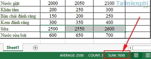
1. How to quickly calculate total using status bar

How to do:

- Select the cells containing the data you want to sum.
- Look at the Status Bar at the bottom corner of the Excel screen.
- The sum will be displayed immediately.

2. How to automatically calculate sum using AutoSum

Advantage:

- Automatically detects data range.
- Fast, no need to enter formula.
- Can be used for both horizontal and vertical rows.

Step 1: Select the blank cell right below the column to be summed.

Step 2: Go to the  Home tab ,  Editing group , click  AutoSum  (∑).

Step 3: You will immediately see Excel automatically add =SUM and select your data column number.

Step 4: Excel automatically selects the data area, press  Enter  to display the results.

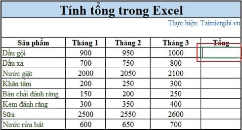
3. How to calculate the total using the SUM function

The SUM function in Excel helps you calculate the total of cells in a column or multiple data ranges flexibly. You can enter the cell address directly or select the data range with the mouse.

Step 1: Click on the cells in your table where you want to see the sum of the selected cells.

Step 2: Enter =sum( into this selected cell.

Step 3: Now select the range with the numbers you want to sum by holding down the Ctrl key and clicking on the data cells then press Enter .

Note: You can enter the addresses manually like =sum(B1:B2000) . It is useful if you have a large range data table to calculate.

After pressing Enter , the sum will appear in the exact cell you selected.

Note:
* With conditional calculation, you only need to apply the following function:  =SUMIF(range, criteria,sum_range)
In which:
- Range: The selected range containing the conditional cell.
- Criteria: The condition for performing the sum function.
- Sum_range: The range to calculate the sum.
* To avoid errors, you need to enter the correct function.

In Excel, there are many ways to sum data, helping you process data quickly and accurately. When you count a list with many repeated values ​​in a column and need to calculate based on the corresponding value in the adjacent column, you can use the SUMIF function. This is an effective way to summarize data based on conditions. If you do not know how to use this function, you can refer to the detailed instructions from Free Download.

During the calculation process, many people encounter errors such as the SUM function not working or the result is 0. Don't worry, see the instructions to fix the SUM function error of 0 to fix it quickly.