Instructions on all types of data hiding in Excel are extremely useful

Part 1: How to hide formulas and comments in Excel

In life and at work, there are always hidden things that we want to hide, want to keep secrets from the eyes of others.In Excel, too, there will come a time when you want to hide a formula to hide the profession;a photo, a comment that does not want others to know;or even hide the whole sheet or entire Excel file so that no one can find it.The problem is how to do it, you do not need to worry, becauseTipsMakewill guide you all the types of data hiding in Excel in a specific, clear and most detailed way.

The followingTipsMakewould like to use the version of Excel 2007 to guide you.As long as you understand the nature, we believe that you will be able to apply it to all different versions of Excel.The article will be divided into several parts, in this part, Accountant Duc Minh will show you how to hide formulas and comments.

1) Hide formulas in Excel

Let us give you an example where you want to hide the formula in cell C13 as shown below:

Instructions on all types of data hiding in Excel are extremely useful Picture 1

- Step 1: You select a cell (cell) or cells to hide the formula, in this case cell C13, then go to 'Format Cells'. There are two ways: press 'Ctrl + 1' or right click and select 'Format Cells'.
- Step 2: Go to 'Protection' and tick the 'Hidden' checkbox if it is not already ticked.

Instructions on all types of data hiding in Excel are extremely useful Picture 2

- Step 3: Go to the ' Review ' tab -> select the ' Protect Sheet ' item in the ' Changes ' group, a ' Protect Sheet ' dialog box will appear, enter the password to be protected in the ' Password to unprotect sheet ' text box. Then click ' OK ' and re-enter that password into the ' Reenter password to proceed ' text box -> ' OK '.

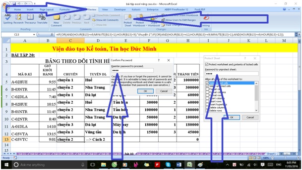
Instructions on all types of data hiding in Excel are extremely useful Picture 3

Now, when you select cell C13 to see it you won't be able to see the formula anymore, but the value in cell C13 as ' trip 2 ' still exists.So you have succeeded.

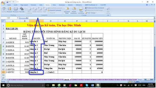
Instructions on all types of data hiding in Excel are extremely useful Picture 4

2) Hide comments in Excel

By default, when you create a comment in Excel, any cell with a comment will show a red triangle in the top right corner of the cell.And when you hover over or select the box, those comments will appear.

Now TipsMake would like to give an example of you want to hide a rather sensitive comment ' She is my lover!'about an image in Excel as shown below:

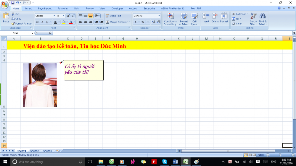
Instructions on all types of data hiding in Excel are extremely useful Picture 5

So you need to follow these steps:
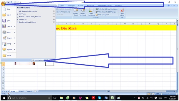
- Step 1: Left-click the Microsoft Office Button (the icon in the top left corner of Excel 2007), then select 'Excel Options' (In Excel 2010 and Excel 2013 go to File -> Options).

Instructions on all types of data hiding in Excel are extremely useful Picture 6

- Step 2: Choose ' Advanced ' -> scroll down to find ' Display ', then left click on ' No comments or indicators ', then click ' OK '

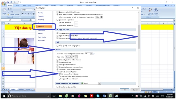
Instructions on all types of data hiding in Excel are extremely useful Picture 7

-> And here is the result:

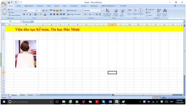
Instructions on all types of data hiding in Excel are extremely useful Picture 8

* Note: Comments will only appear once you turn on the ' Show All Comments ' mode in the Review tab.

Part 1: How to hide formulas and comments in Excel, this series of articles about hiding data types in Excel is over. Tipsmakewish you success and see you in the following sections, promising many interesting things.

Samuel Daniel

Update 13 April 2020

You should read it

May be interested

How to import data from photos into Excel
on the office 365 version, users can already import data from photos into excel for immediate use without having to find some data extraction tools from photos. users can extract data from photos into excel with saved images or from screenshots.
Steps to use Pareto chart in Excel
pareto charts in excel are also commonly used in excel with other excel chart types. this chart type is created from the pareto principle, including vertical bars and horizontal lines to represent data in excel data tables.
MS Excel 2003 - Lesson 2: Format spreadsheet data
tipsmake.com will guide you how to format data in excel 2003, detailing font options, data types, how to align data in cells, spreadsheets.
Forgot password protected Excel file, what should you do?
suppose in case if there is an excel file containing extremely important data and because you want to keep your data secret, you create a password for the excel file to ensure its safety and data protection. file. however, for a long time not to use, forgetting passwords is also common.
How to Automatically Report on Excel
today's tipsmake will guide you how to automatically report data on microsoft excel. this article also talks about how to query and create reports from external sources (mysql, postgres, oracle, etc.) right on your spreadsheet using the excel plug-in to link your spreadsheet to the source. that data. as for data stored on excel spreadsheets, we will use macro commands to create and export reports into many different file types with just one keystroke. luckily, excel has this feature built in, so you won't need to create your own algorithm.
Summary of data in groups in Excel
instructions on how to aggregate data in groups in excel. with a large amount of data, statistical data is very complicated. here, with excel 2013, the subtotal feature helps you to aggregate data by group, giving a detailed, complete and accurate report.
How to copy data from Excel to Word?
in some cases you need to insert some data into word documents to make reports, presentations ... the following article the network administrator will guide you how to copy data from excel to word.
How to take screenshots with Excel is extremely simple
to take an excel screenshot, you will use the tool available right on excel to take a screenshot of the data table, or even take a screenshot on your computer to insert the image into excel.
MS Excel 2003 - Lesson 3: Manipulating data in spreadsheets
the previous article tipsmake.com has guided you to some basic formatting for a small data area, but if you need to format a large area or the default format for a new excel 2003 file, follow these instructions.
How to sort data in Excel using Sort is extremely simple
with just a few operations to arrange data in excel, you can transform your spreadsheet to become neat and easy to see. let's find out with free download now!