How to use the UNIQUE function in Google Sheets

Usually, we import data into our spreadsheets from different sources. Whether online or from other software, there are bound to be instances where data is duplicated. In these cases, you will need to clean up your data to remove duplicate values, which can become very tedious to do manually.

In these cases, using the UNIQUE function in Google Sheets is a smart choice. This article will discuss the UNIQUE function, how to use it and combine it with other functions.

Hàm UNIQUE trong Google Sheets là gì?

Hàm UNIQUE trong Google Sheets là một hàm tiện dụng giúp bạn tìm các giá trị duy nhất trong tập dữ liệu đồng thời loại bỏ mọi dữ liệu trùng lặp.

Hàm này lý tưởng nếu bạn thường xuyên làm việc với một lượng lớn dữ liệu. Nó cho phép bạn tìm các giá trị chỉ xuất hiện một lần trong bảng tính. Nó hoạt động tuyệt vời cùng với các kỹ năng và hàm quan trọng khác của Google Sheets. Công thức của hàm UNIQUE sử dụng ba đối số, nhưng phạm vi ô là đối số cần thiết duy nhất.

Cú pháp cho hàm UNIQUE trong Google Sheets

Đây là cú pháp cần làm theo để sử dụng hàm UNIQUE trong Google Sheets:

=UNIQUE( range, filter-by-column, exactly-once)

Đây là những gì mỗi đối số đại diện:

1. range - đây là địa chỉ ô hoặc dải dữ liệu mà bạn muốn thực thực thi hàm trên.
2. filter-by-column - this argument is optional and you use it to specify whether you want the data to be filtered by column or row.
3. exactly-once - this is also an optional parameter and determines if you want non-duplicate entries. FALSE means you want to include unique values. TRUE means you want to remove entries with any number of duplicates.

To use formulas, make sure that you format the numeric values ​​correctly.

How to use the UNIQUE function in Google Sheets

Here are the steps you need to follow to use the UNIQUE function in Google Sheets:

How to use the UNIQUE function in Google Sheets Picture 1

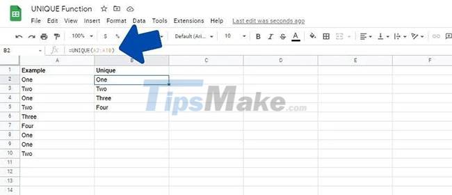
1. 1. Click the blank cell where you want to enter the formula.
2. 2. Type =UNIQUE( to start the formula.
3. 3. Type or click and drag across the appropriate range of cells.
4. 4. End the formula with a closing brace.
5. 5. Press Enter to execute the formula.

Here is another example to demonstrate the UNIQUE formula.

How to use the UNIQUE function in Google Sheets Picture 2

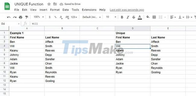
This example works with two columns instead of one. When executing the formula in the data, the formula will search for unique values ​​in two columns at the same time instead of searching each column.

You can observe this as Ryan Gosling and Ryan Reynolds. Although the two share the same name, they are unique, meaning the two values ​​are separate. Learning this function will also help you master the UNIQUE function in Excel.

Combine UNIQUE . function

Similar to most other functions in Google Sheets, the UNIQUE function can be paired with other formulas to enhance its functionality. Here are a few ways you can do this.

UNIQUE with SORT

How to use the UNIQUE function in Google Sheets Picture 3

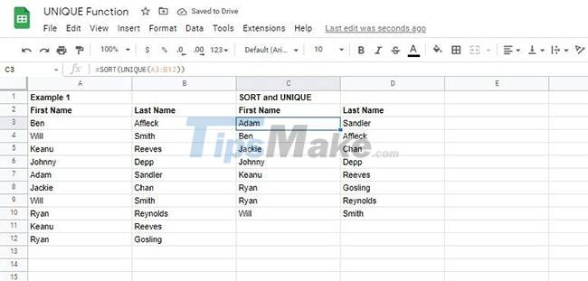
The article used one of the previous examples here. Using a UNIQUE formula with two columns provides the expected result. Now, use SORT with UNIQUE to find unique values ​​in the dataset and sort them alphabetically.

UNIQUE with TRANSPOSE

How to use the UNIQUE function in Google Sheets Picture 4

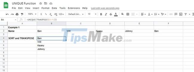
You can only use the UNIQUE function with vertical data, so you will need to convert the horizontal data to vertical before using the UNIQUE function on it. TRANSPOSE in Google Sheets works similarly to Transpose in Excel. So you can use it to lay your output horizontally.

Make sure there is space required for the data to be displayed before writing the formula. If you want to convert the data back to its original form, use the TRANSPOSE function again.

Tips for UNIQUE . function

Here are some tips for using the UNIQUE function in Google Sheets:

1. Make sure you provide enough space for the data set's contents to be displayed. If the data cannot fit in the space provided, Google Sheets will display the #REF! error.
2. If you want to clear all values ​​that the UNIQUE function displays, delete the first cell where you enter the formula.
3. If you want to copy the values ​​returned by a UNIQUE formula, copy them first with Ctrl + C or by right-clicking, clicking, and selecting Copy. To paste the values:

1. Click Edit

2. Then go to Paste and Paste Special .

3. Click Paste values ​​only . The formula will be deleted and only the values ​​will be retained.

The UNIQUE function is a simple yet convenient function to use in Google Sheets, especially if you work with large spreadsheets.

You can use this function and many other Google Sheets features to calculate and make important business decisions.

Samuel Daniel

Update 10 May 2022