How to Acquire Slant Parabolas in Excel

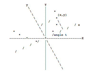
Take the familiar equation y = Kx^2 and rotate it about the origin.

Do this by making a substitution of two new variables (X and Y) using equations like this:

1. x = cos(t)*X + sin(t)*Y
2. y = -sin(t)*X + cos(t)*Y
3. where sin and cos are the sine and cosine functions from trigonometry, and t is the angle by which you are rotating the parabola, and where you'll let X and Y vary between -5 and 5, being sure that 0 is one of the values as well.

Start by opening a new workbook in Excel from the desktop, from the dock, or from within your Applications folder inside the Microsoft folder. Double click on Excel (either the green X on the dock or the app title in the folder) and select File New Workbook.

Click in the far upper left top corner above the 1 of row 1 and to the left of column A. Doing so will select the entire worksheet. Format Cells Number Number to decimal places 2, show comma. Format Cells Alignment Center.

Enter the Row 1 Column Headers:

1. Enter to cell A1 the label, Factor1. The cell beneath it will become the Defined Named Variable Factor1, which will be used to factor the parabola's size of the x coordinate, e.g. if you want to cut all the x values in half, you would enter .5 into cell A2;
2. Enter to cell B1 the label, Factor2. This will be used to factor the y coordinates.
3. Enter to cell C1 the label, ParaVertex X. Used to control the vertex.
4. Enter to cell D1 the label, ParaVertex Y. Also used to control the vertex.
5. Select cell range A1:D2 and Insert Name Create Names in Top Row. This will assign the labels as Defined Variable Names to the cells A2 to D2.
6. Enter to cell A2 the value, 1;
7. Enter to cell B2 the value, 1;
8. Enter to cell C2 the value, 5;
9. Enter to cell D2 the formula, =5+5-1.79; (w/o the ending semi-colon)

Enter the Row 3 Column Headers:

1. Enter to cell A3 the label, Chart x;
2. Enter to cell B3 the label, Chart y;
3. Enter to cell C3 the label, angle t;
4. Enter to cell D3 the label, cos(t);
5. Enter to cell E3 the label, sin(t);
6. Enter to cell F3 the label, X and Y Series and Format Column Autofit Selection;
7. Enter to cell G3 the label, K. Select cell range G3:G4 and do Insert Name Create in Top Row. This will create the defined variable name K for cell G4, which can now be used in a formula. Select cell G4 and enter the value 5 into it.

Enter the formulas and series for the short data section to be charted:

1. Enter to cell A4 the formula, =ParaVertex_X+Factor1*K*((D4*F4)+(E4*F4))^2; do Format Cells Fill Yellow and copy it and paste it to cell A5;
2. Enter to cell B4 the formula, =ParaVertex_Y+Factor2*((-E4*A4)+D4*F4); do Format Cells Fill Yellow and copy it and paste it to cell B5; the minus sign is important -- please don't miss it;
3. Enter to cell C4 the value 40 and enter to cell C5 the formula, =C4;
4. Enter to cell D4 the formula, =COS(C4*PI()/180);
5. Enter to cell E4 the formula, =SIN(C4*PI()/180);
6. Copy cell range D4:E4 and paste it to cell range D5:E5;
7. Enter to cell F4 the value -5;
8. Do Edit Fill Series, accept the default Step Value of 1, for cell range F4:F14 -- you should have the value 0.00 in cell F9 and the value 5.00 in cell F14;
9. Copy cell range A5:E5 and Paste it to cell range A6:E14.

Select cell range A4:B14 and do either Insert Chart or from the Ribbon, select Chart, or do Chart Wizard. Do Charts, All, Scatter, Smooth Lined Scatter. A chart will appear atop your worksheet. Drag it off to the right just past the data, out of the way, then hover over the bottom right corner until the cursor turns into a double-headed arrow, then pull the chart down and to the right to expand it.

1. Your chart should show a very thin parabola, like the fiber of an iris muscle of the eye somewhat, extending from about {5,5} down to {253.10, -158.31} on the left branch and to {253.10, -158.65} on the right branch. It's good that it's so thin, but it's much too long in the x direction to use within our eye & iris chart; we need to factor the x coordinate by 253.1*n = 6 or so, so n = 6/253.1 -- perform that computation by entering it below the data as =6/253.1, and then copy it and paste it to cell A2;
2. Now the parabola is still slanted, which is what you want, and which is dependent on both the size and plus or minus status of angle t and value K ... but it is now too wide open, and the vertex has shifted from where it's being reported at {5, 5} slightly;
3. By taking the total difference of the max and min of the y values in column B, i.e. 5.93- -2.61, you arrive at a total height of the curve of 8.55; you want it to be more like .55, so you create another little formula algebraically to adjust Factor2, which is .55 = n*8.55, so you enter =.55/8.55 into cell B2;
4. The curve still displays as wide, but that's because Excel shortened the y scale range of the chart dramatically. Click on the vertical axis and set the maximum to 10 and the minimum to 0.0 -- there now, that's better. And the iris fiber extends out to the right about 5 units. But its vertex has moved up to {5, 8} and you want it more like {5, 5} (we can be more exacting later), so you need to subtract 3 from ParaVertex_Y in cell D2 -- do so now.
5. OK! Success! That's beginning to look like where you want to begin your iris fibers!
6. Try doubling the angle t to 80 -- see how thin it gets? You would think that, since 80 degrees is twice the angle that 40 degrees is, the opposite effect would have occurred, but now try half of 40, 20 for angle t in cell C4. It widens the parabola instead of thinning it. The reason for that is all the constraints we've put on the curve in this author's opinion. Nor is the curve any longer at much of a slant, but falls pretty much along the x axis. Clearly, this is going to take some tinkering with to be useful but there it is, in the rough, the slant parabola.
7. Change K to .09 and watch the X scale become a great deal shorter in fact. This means you are now capable of creating "cascading parabolas", though not yet in a fractal, multiple way. That will come with the next article, hopefully! Enjoy!

Try the following changes to angle t, by manually inputting them:

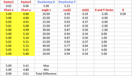
1. Here's an image of the data chit of the worksheet just completed (and including the Tips below):
   How to Acquire Slant Parabolas in Excel Picture 3
2. Here's an image of the chart where we just ended up, after adjusting Curve Smoothness:
   How to Acquire Slant Parabolas in Excel Picture 4
3. Here's a data chit with another series added, for making two parabolas on the chart (it uses the Angle t to vary the curve):
   How to Acquire Slant Parabolas in Excel Picture 5
4. Here's a chart of the two parabolas, one more curvy, the other more slanted (the red is the lower data, the blue is the upper data):
   How to Acquire Slant Parabolas in Excel Picture 6