106 tips with Microsoft Office - Part 7

106 tips with Microsoft Office - Part 7 Picture 1 Microsoft Excel

One page - A chart

Usually the charts will come with data related to it. But sometimes you want to print that chart out of a completely separate page, separate from the data. Very simple, select that chart and then go to File | Print, the chart will be printed on a separate page.

The chart only has 2 black-white colors

Another convenient feature when you print a chart in Excel is the Preview command. Even if you have a color printer, you can still print charts with only black and white by going to File | Print then select the Preview button. In the Preview window, select the Setup button and select Chart, select the option before Black and white. Now in Preview Preview section your chart is displayed in 2 black-and-white colors to make it easier to adjust the contrast of the bars, lines or columns of the chart.

The file name is printed in Footers

  106 tips with Microsoft Office - Part 7 Picture 2 Starting with Excel 2002, Microsoft has added the ability to insert the path of a spreadsheet file into Header or Footer. This path also automatically updates when you move the file. To insert a spreadsheet file path into Header or Footer, please follow the following way:

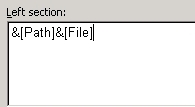
Go to View | Header and Footer or File | Page Setup | Header / Footer, select Custom Header or Custom Footer. In the Custom Header or Custom Footer window, select the location where you want to name the lead of the file - on the left, right or center. Place the cursor in that position and click on the folder icon in the toolbar just above. At that location, you will see the code [[]] & [File]. So successful.

Confirm information

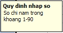  106 tips with Microsoft Office - Part 7 Picture 3 If faced with a spreadsheet with many different types of data, it is very easy to confuse processing data. To avoid confusion you can use the Confirm Information feature in Excel.

For example, if you have a tax column and are sure that the tax does not exceed 100%, then you can specify that Excel only accepts values ​​less than 100. So if you miss it, you will not be confused, Excel will remind you Remember to not exceed 100. Or you can set a value within a certain range . You can set the Data Validation for a cell, a range of cells, a row of a column .

To use this feature in Excel, first select the cell - row - column that wants the application to confirm the information later on Data | Validation. You give your input rules and click OK.

If you send spreadsheets to others, you should put additional comments for cells - rows - columns that have the Data Validation application so they can enter the correct information in the following way.

In the Data | Validation you go to the Input Message, naming and commenting clearly. So every time the cursor is moved to the cell with the Data Validation feature, it will show specific instructions for users.

Similarly, you can fully customize the warning when entering the wrong data by going to the Error Alert field to enter the name and alert content into it.

Customize the list

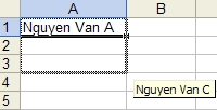  106 tips with Microsoft Office - Part 7 Picture 4 If you often have to enter the same data type on different spreadsheets - for example, a list of company employees - you can use Custom Lists to speed up and simplify this work.

Go to Tools | Options then go to Custom Lists. In the window that appears, select New List in the left-hand pane, and in the right-hand pane you enter the values ​​in your list into it, each of the objects in the list is one line, finally you select the button Add. Or if you already have a list, you can select Import list from cell and select the cells that contain the data you want to import the list.

Now you just need to type any object in your list and move the cursor to the lower right hand corner of the cell until the pointer changes to a plus sign and drag to the cells you want the list to appear on. out.Excel will help you fill in the remaining values.