Coloring Alternating Excel Lines Not Everyone Knows

Sometimes the plain Excel template tables are just plain white and can be very confusing. To help readers overcome this and can look up necessary information as quickly as possible without confusion. Simply with the following 5 steps for you to color alternately for rows in Excel spreadsheets!

Step 1:

You press Ctrl + A or you can press the triangle button on the left corner of the sheet to highlight the entire Excel table.

Step 2:

Then you go to Home, in Slyle select Conditional Formatting, select New Rule.

Step 3:

Then the New Formatting Rule dialog box appears. You select Rule Type:Use a formula to determine which cells to format In the Format values where this formular is true box, type the formula: = MOD (ROW (), 2)> 0

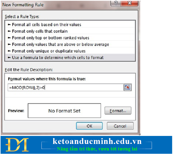
Step 4:

When you click Format, the Format Cells dialog box appears.

On the Fill tab, select the color you want, then select OK.

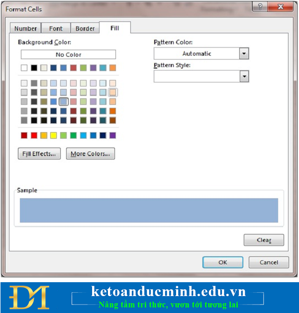
Step 5:

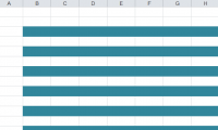
After you press OK, let's see the results achieved offline!

It's simple and fast, with 5 super-fast steps that can help you differentiate between different viewing lines in Excel.