4 Basic Steps to Color Alternating Lines in Microsoft Excel

The following guide provides a clear overview of Excel 2013, with the most relevant background, details, and practical takeaways.

Excel 2013 Overview

Step 1:

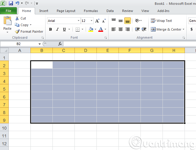
Open the Excel spreadsheet and then black out the lines to fill, as in the example here I select the rows, column Excel from B2 to H9:

Step 2:

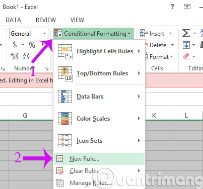
On the menu bar, click the Conditional Formatting item, select New Rule.

Step 3:

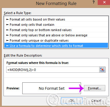
When the New Formatting Rule dialog box appears, click the Use a formula LINE to determine which cells to format and then enter the following formula LINE in the Format values ??where this formula field is true: = MOD (ROW (), 2)> 0. Then click Format.

Step 4:

When the Formatting Rule dialog box appears, click the Fill tab and select the desired color.

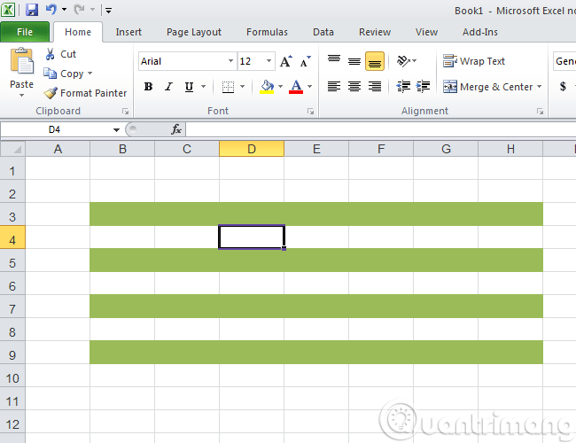
Click OK, and we will have the Excel cells colored alternately as shown below:

Step 5:

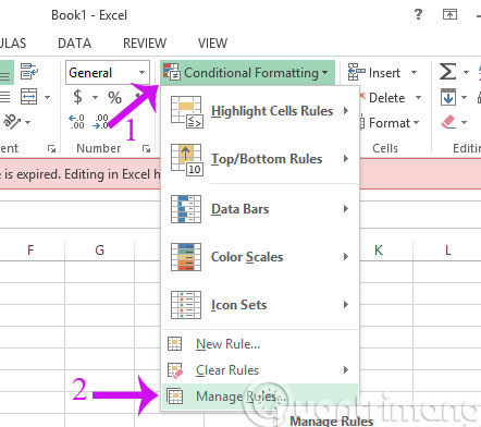
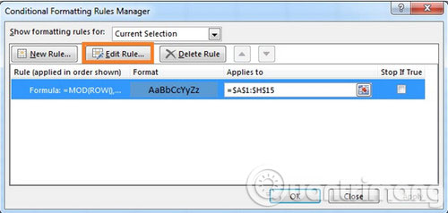
If you want to change to another color, click on the Conditional Formatting section and select Manage Rules.

Step 6: When the new dialog appears, click Edit Rule

Step 7: Click the Format button to change to the desired color

So, you already know how to color between Microsoft Excel lines. This job is small but it will contribute to minimizing errors in the calculation process for you.

• How to convert numbers into words in Excel?
• So what if you want to interleave color data in Excel?
• The most basic functions in Excel
• How to keep the cells fixed in Excel?

Good luck!