14 time-saving tips when using Microsoft Excel

Microsoft Office Excel spreadsheet application is a powerful, fully-featured tool for working with complex spreadsheets, statistics, tracking and reporting. With the number of commands, the huge feature will take a lot of time to be able to use proficiently, but if you understand some of the tips below will greatly reduce the time when working on Excel.

Actions and tips in this article are done on Microsoft Excel 2016 - Microsoft's latest spreadsheet application.

1. Use the template

One of the best time-saving ways for most tasks is to use templates. You can use them in Microsoft Word to serve agendas, newsletters or reports. In Excel, templates are even more useful. For timeline projects, calendars, invoices, budgets and more, taking advantage of these extremely convenient, pre-formatted tools will definitely save a lot of time and effort.

Collecting the necessary spreadsheet templates is as easy as using them. Microsoft website provides a variety of different Excel templates for calendars, plans, tracking tools, time tables, etc. Vertex24 has many interesting sample options for calendars, budgets, to-do lists and balance sheet. A huge source of Excel templates for invoices, inventory, login form, . is Spreadsheet 123.

14 time-saving tips when using Microsoft Excel Picture 1
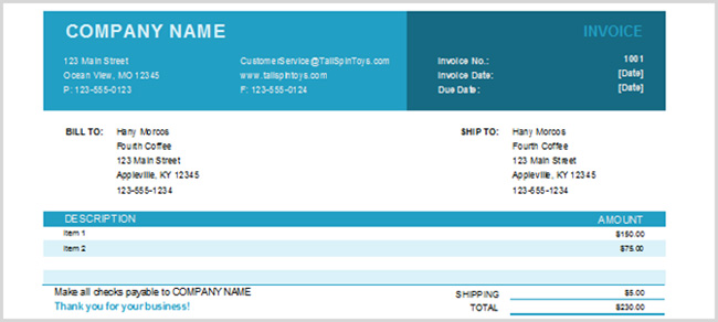
A basic invoice template is created in Excel

2. Fixed rows and columns in Excel

If there is a long table containing tons of data, you may have to scroll your mouse down or up for a long time to be able to find the area you need, but when you find the data you don't know what it is, because the subject line is not can see. This takes a lot of time when you have to drag up and down continuously to see the title of the data. However, if the rows and columns freeze, the titles will remain the same when moving the mouse in the spreadsheet.

Go to the View tab > Freeze Panes on the Ribbon. In the Freeze Panes drop-down menu, select Freezze Panes (freeze both the top and first rows), Freeze Top Row (freeze the top row of the spreadsheet), Freeze First Column (freeze the first column of the spreadsheet) ).

14 time-saving tips when using Microsoft Excel Picture 2

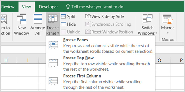
Now, when you scroll your mouse down, up, right, left, you will see frozen columns and rows that are not moving and always within sight. To cancel freezing these rows and columns, simply select the Freeze Panes command again and click Unfreeze Panes .

Note: For older versions of Excel, the above process may vary slightly. Select the common box for both rows and columns to freeze, then click Freeze Panes .

Explore more:

1. How to keep the cells fixed in Excel?
2. Video tutorial using Freeze feature - fixed column, line in Excel

3. Use the Fill Handle

A Fill Handle is a black dot that appears in the lower right corner when selecting one or a group of cells in a column. Knowing how to use the Fill Handle will save you tons of time when you need to fill in data like sequential numbers, days, months and years in a row. There are several ways to use the Fill Handle.

First, you can quickly create a list of counts by entering 1 in the first box, 2 in the box below it, then selecting both cells, the Fill Handle appears, drag down the cells below until reach the desired number. It is not necessary to fill in 1, you can make any number like 15, 20, but it can only create a continuous, progressive sequence. That is, if you enter 15, you will create lists from 15, 16, 17, 18, .

14 time-saving tips when using Microsoft Excel Picture 3

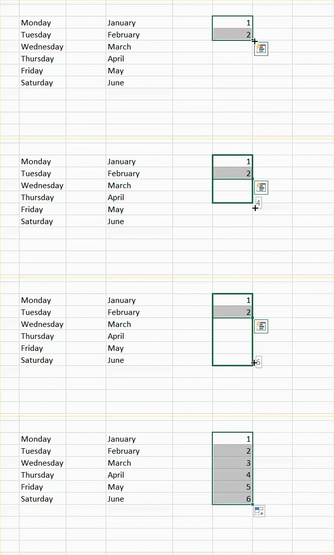
When using this feature for dates, just fill in a date any day like 05/01/2017, select that box and scroll down, Excel will automatically increase the date exactly as the calendar. This operation is also applicable when creating columns for months of the year or days of the week.

14 time-saving tips when using Microsoft Excel Picture 4

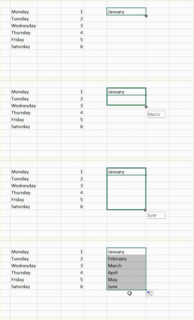
Another useful use is when you need to enter the same value into the entire column in the spreadsheet. For example, fill in the letter A, select the box and double-click the Fill Handle. This will enter the A value for all the remaining cells of the column in the spreadsheet.

4. Switch between columns and rows

If you have a spreadsheet that uses headings in columns or rows (or both) and thinks that when changing columns for rows, the spreadsheet will be more intuitive, use this tip to make it quick and easy. It saves you more time without having to retype titles.

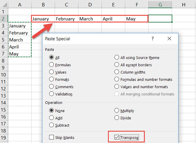
Here are the steps to move cells from the title row to the title column:

1. Select the cells in the column that contains the title
2. Right-click, select Copy or click the Copy button on the Home tab of the Ribbon
3. Select the cell in the row and column you want the titles to start.
4. Right-click and select Paste Special or click Paste> Paste Special on the Home tab of the Ribbon
5. Check the Transpose checkbox in the lower right corner
6. Click OK and see the result

14 time-saving tips when using Microsoft Excel Picture 5

Further reference: Convert lines to columns in Excel

5. Access the computer

Besides supporting external computer add-ins, Excel also has a built-in calculator feature, so if you don't want to install additional add-ins, you can take advantage of this available computer. This will be convenient in case you want to quickly calculate calculations that are not built in spreadsheets.

Excel allows you to add computers to both the Ribbon and the Quick Access toolbar.

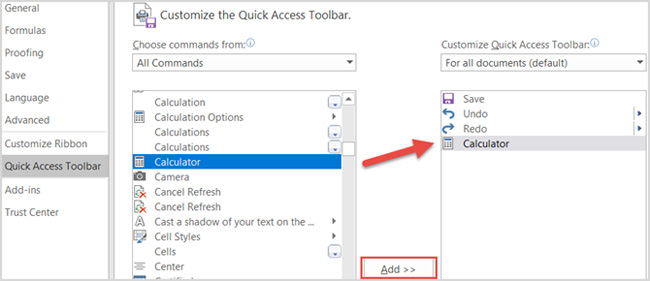
To add a computer to these two locations, start by selecting File> Options . Then, select Customize Ribbon (add a computer to the Ribbon) or Quick Access Toolbar (add Quick Access), depending on the location you want.

In Choose commands from:> All Commands> Calculator and click Add >> to add the computer to the Quick Access toolbar. If you add a Ribbon, you need to create a custom group and then add the computer to it.

14 time-saving tips when using Microsoft Excel Picture 6

6. Link tabs or columns

If your Excel file contains multiple spreadsheets with data that are cross-referenced between them, creating a direct link will provide faster access. This is especially useful if you need to share spreadsheets with others so they can move to referenced data quickly.

Follow the simple steps below to create links:

1. Select the cell containing the data you want to link
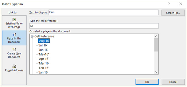
2. Right-click and choose Hyperlink or go to the Insert tab, select Hyperlink
3. In the pop-up window that appears, select Place in this Document
4. Then enter the text to display in that cell, enter a specific cell reference if desired and the worksheet in Excel file with data linked to
5. Click OK

14 time-saving tips when using Microsoft Excel Picture 7

7. Use Excel keyboard shortcuts

Regular use of shortcuts when working on Excel is definitely an effective time-saving solution.

You can refer to more Excel shortcuts than in the article: Summary of shortcuts for Microsoft Excel 2016-P1

Here are some shortcuts that can significantly speed up your work:

1. F4 or Fn + F4 to repeat the last command, including changing the format like color or font
2. Alt + H, E, A to delete the content, format and other attached data in the selected cell
3. Ctrl + W to close the spreadsheet and Ctrl + O to open the new table
4. Ctrl + Shift +: (colon) to enter the current time and Ctrl + Shift +; (semicolon) to enter the current date
5. Shift + F9 to calculate active spreadsheets
6. Shift + Tab to move to the previous box or option
7. Ctrl + Home to move to the top of the spreadsheet
8. Ctrl + Page Down to move to the next table in an Excel file and Ctrl + Page Up to move to the previous worksheet

8. Working with AutoSum

14 time-saving tips when using Microsoft Excel Picture 8

Some people may think that working with Excel formulas is too time consuming. But even for simple equations, these built-in functions can definitely help users manipulate faster.

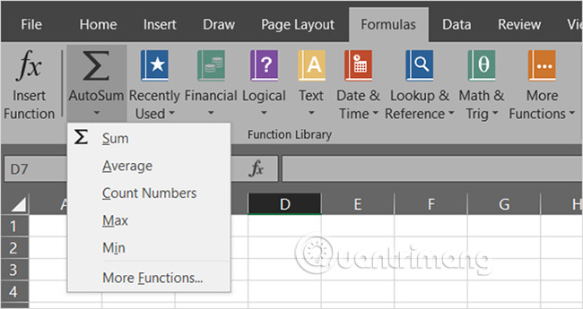
Unless you have moved or deleted it from the ribbon, the AutoSum button will be on the Home tab . This handy feature provides users with the most popular formulas with one click. You can add, count or calculate an average for a group of numbers or find the number with the maximum (max) or minimum (min) in that set. Just click the arrow on the AutoSum button to select the formula you need.

In addition to the AutoSum feature , the Formulas tab also contains more options. Each recipe is placed in a specific category so that users can easily search. You can choose from functions related to finance, logic, math, statistics or engineering.

But for the commonly used formulas, AutoSum feature is very quick and convenient.

9. Using Conditional formatting is simple

14 time-saving tips when using Microsoft Excel Picture 9

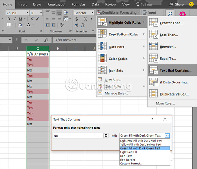
Conditional formatting is one of the other Excel features that many people find a little intimidating. However, for data with special data, it is a great tool.

For example, you have a data sheet from a survey and want to see how many Yes answers and how many No answers immediately. Please apply the following steps:

1. Select the boxes containing the answer Yes / No.

2. On the Home tab , click the drop-down Conditional Formatting box.

3. Select Highlight Cells Rules and then Text That Contains .

4. Enter the word Yes in the left box and select the format from the box on the right.

5. Follow the same steps for answer No.

After that, you will see all Yes and No answers formatted in the selected way, so it is easy to see.

If you plan to continue adding data, you can also apply this conditional format to the entire column or row instead of just one group of cells. This way, future data will be formatted automatically as soon as you enter them.

10. Insert chart fast

14 time-saving tips when using Microsoft Excel Picture 10

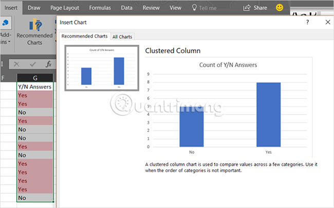
Excel's Charts feature is a great tool for visualizing data. And, you can choose from a variety of different charts such as pie charts, lines, columns, etc.

Using the conditional formatting example for the Yes / No answer above, you can insert the chart with just a few clicks.

1. Select the boxes containing the answer Yes / No.

2. On the Insert tab , click Recommended Charts. With this option, Excel will retrieve the data and include it in the most appropriate chart type.

3. If you like the type of Excel chart that is automatically selected, click OK and it will be inserted into the spreadsheet.

This is the easiest and fastest way to create charts in Excel. This process only takes a minute to complete. However, if you don't like the chart created, you can click the All Charts tab in the pop-up window and experiment with other chart types.

11. Arrange with filters

If there is a spreadsheet containing multiple data columns, you may want to sort or filter all the information by a certain column. Although there are several ways to do this, using filters is still the fastest and safest way.

1. Select the entire sheet by clicking the triangle button next to the first column on the top left.

2. On the Home tab , click Sort & Filter .

3. Select Filter.

This step will make an arrow appear in the first row of each column. When clicking on the arrows, the user can sort the entire sheet in the way that has been chosen to sort that column. If it is a date field, the user can sort from the oldest to the latest and if it is a text field, can sort alphabetically.

In addition, users can filter data to view only the items you want. When clicking on an arrow, you will see check boxes next to the items. Checking or unchecking these boxes will filter the data, helping you see exactly what you need.

14 time-saving tips when using Microsoft Excel Picture 11

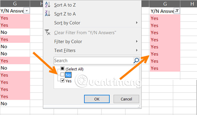
The great thing about using the Filter feature is that it doesn't negatively affect the rest of the data. If you want to sort the entire sheet, Excel will adjust all columns. And if you want to filter, Excel will only hide what users don't want to see.

12. Use Format Painter

If you already use other Microsoft Office applications like Word, you may be familiar with Format Painter. In Excel, this handy tool allows you to apply the same format from one or more cells to other cells with one click.

1. Select the cell, group of cells, rows, or columns that you want to copy the format from.

2. On the Home tab , click Format Painter.

3. Select the cell, group of cells, rows, or columns that you want to copy the format.

This is a great way to quickly apply the format of these cells to other cells without manually manipulating them.

13. Convert and view windows

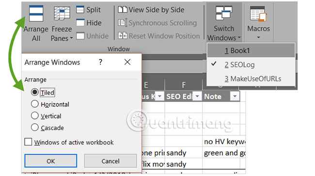
Do you ever need to work with multiple Excel windows at the same time? You may need to review the data, compare it or even copy data from one workbook to another. Excel provides a useful feature set to help with this. Look to the View tab to check these options.

1. Arrange All: When you click this button, you can arrange all your open workbooks on one screen. Choose a horizontal, vertical or cascading view as you like.
2. View Side by Side : This option allows you to select two open workbooks to be placed side by side or stacked, very suitable for comparison.
3. Switch Windows: Click this button when you open multiple Excel workbooks at once and want to quickly switch between them. No need to maximize or minimize the windows with this great feature.

14 time-saving tips when using Microsoft Excel Picture 12

14. Install handy add-ins

Office add-ins are similar to browser extensions in that they are tools to enhance the experience, data and efficiency for the application. And in Excel, you have many useful add-ins to choose from.

Select the Insert tab and click Store. You can then check the tools by category. For example, the Productivity category contains add-ins to automate documents and template library templates. And the Project Management category has add-ins for Gantt charts and active timers.

14 time-saving tips when using Microsoft Excel Picture 13

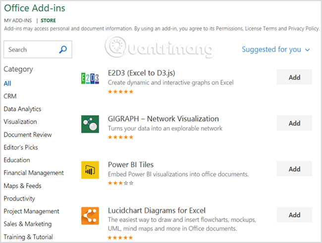
Some add-ins are free, while other add-ins require payment, so be sure to check the details before installing.

The above are just a few small tips to help readers save time when using Microsoft Excel. TipsMake.com will continue to find more good tips when using Excel. If you like and regularly use Excel, you can contribute the time-saving tips I've found and share with everyone in the comment section below the article.

See more:

1. How to add computers to Excel
2. You want to print text, data in Microsoft Excel. Not as simple as Word or PDF! Read the following article!