4 basic steps to color alternating columns in Microsoft Excel

In the previous article, TipsMake.com showed you some basic steps to color alternate cells, different data streams in Microsoft Excel. But what about the data column? Many of you have asked such a question, please join us in solving this problem.

See more articles:

1. How to color alternate cells and rows in Micosoft Excel

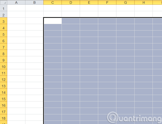
Step 1:

Drag the mouse and select the columns of data to color, as in this example, from C3 to G19:

4 basic steps to color alternating columns in Microsoft Excel Picture 1

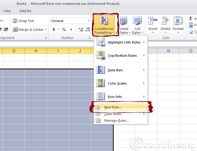
Step 2:

Select menu Home> Condition Formatting> New Rule:

4 basic steps to color alternating columns in Microsoft Excel Picture 2

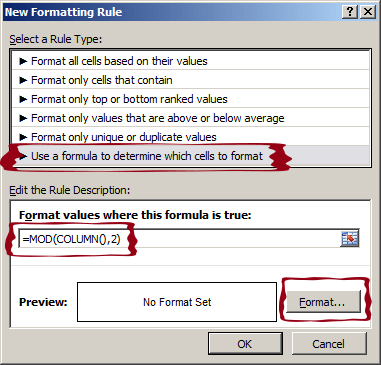
Step 3:

The New Rule table displays, you select:

1. Dùng một đối thức đến dertermine mà cơ sở dữ liệu để định dạng

In the box:

1. Format values ​​where this formula is true

We enter the formula:

= MOD (COLUMN (), 2)

Then, select Format to fill the color:

4 basic steps to color alternating columns in Microsoft Excel Picture 3

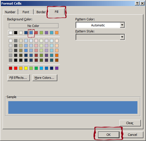
Step 4:

The Format Cells table displays, select the Fill section as shown below. Select the color you want to fill into the different columns in the Background Color section, then click the OK button:

4 basic steps to color alternating columns in Microsoft Excel Picture 4

And this is our result:

4 basic steps to color alternating columns in Microsoft Excel Picture 5

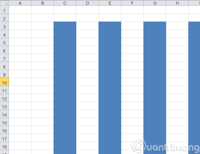
If you want the Excel worksheet columns to return to normal, do the same as above, apply the columns you want to select, then Home> Conditional Formatting> Clear Rule. The above is a simple trick that makes it easier to master Microsoft Excel spreadsheets, avoiding confusion when entering data, and managing information. Good luck!