Basic Excel functions in accounting

Functions in Excel are no longer a strange concept to Excel users, whether new or old. Using functions in spreadsheets is a daily task for accountants in calculating and recording data, including payroll.

Basic Excel functions in accounting

Using basic accounting functions is one of the first requirements for job applicants in related fields. So what are these basic accounting functions, and are they difficult? TipsMake will now introduce you to the most basic Excel functions for accounting, helping you easily get acquainted with and enjoy Excel more.

Basic Excel functions in accounting

IF function - conditional function

The IF function in Excel is very commonly used; it's a conditional function used to retrieve desired values ​​from a range. It's also a fundamental function in accounting that you need when you want to retrieve data based on conditions. Follow the instructions below to learn how to use the IF function.

Syntax: IF(Logical_test, Value_if_true, Value_if_false).

Logical_test is the condition you set for the string to be evaluated.
Value_if_True/False: is the result displayed if the condition is true (Value_True) and false (Value_Failse).

Explanation: If the condition is true, the result returns the value 1; otherwise, it returns the value 2.

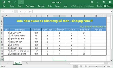
Example: Given a list of 8 students in a class, display the result 'Pass' or 'Fail' if the total score is >= 15, and vice versa.

In this example, we will display the result in cell H6, so the formula to be entered in cell H6 is as follows: IF(G6>=15,'Pass','Fail')

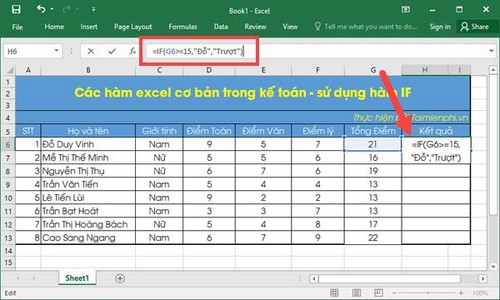
Explanation: G6 corresponds to the Total Score column . Here, we will consider the total score column with a value of >=15 . This will give the results as Pass or Fail , respectively.

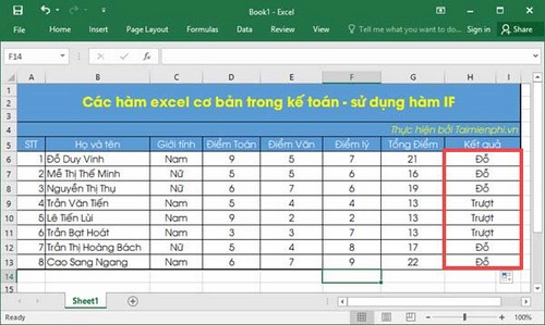
The results are displayed for one column; you can drag and drop the formula to repeat it in subsequent rows. The corresponding results are accurate and you can compare them with the Total Score column .

SUMIF function – a function that calculates the sum based on a given condition.

SUM is a familiar sum function, but a slightly more advanced version is SUMIF, a conditional sum function in Excel. While considered more advanced than SUM, it's still just a basic Excel function used in accounting. Using the SUMIF conditional sum function is very simple; follow the example below.

Syntax: =SUMIF(range, criteria,[sum_range])

Range: The reference string where you will check the IF condition here /
Criteria: The condition applied to the string to be calculated.
Sum_range: The string to be summed.

Explanation: If the values ​​in the Range satisfy the conditions set by the Criteria, those conditions will return the result as a sum.

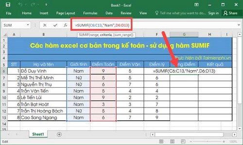
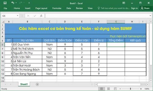
Example: Given a list of 8 students in a class, calculate the total math score of student Nam.

In this example, the problem only asks for the total score of male students in the Math exam, so the column receiving the value is column G(Total Score), the reference column is C(Gender), and the column to be summed is column D(Math Score).

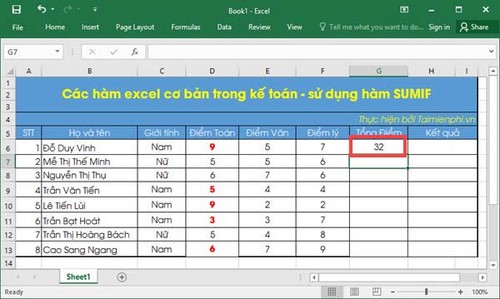
First, we enter the following formula into cell G6: =SUMIF(C6:C13,'Nam',D6:D13).

This corresponds to the column to be referenced, column C (Gender), where values ​​from C6 to C13 must satisfy the condition ' Male '. After the values ​​satisfy the condition, the remaining values ​​in column C will be summed and taken from column D (Math Score), and the result will be displayed.

The results show that there are 5 male students with math scores of 9, 5, 9, 3, and 6 respectively, and their total score is 32.

COUNTIF function – a function for counting based on a condition.

This is a conditional counting function in Excel; it counts the quantity after you apply a condition to the string. Using the COUNT function in Excel is very simple, so the COUNTIF function is also not difficult for users. If you master the COUNTIF function in Excel, combining it with other basic accounting functions will be very convenient.

Syntax: =COUNTIF(range, criteria)

Range: The reference string where you will check the IF condition.
Criteria: The condition applied to the string to be evaluated.

Explanation: This function will count the total number of items in the string you need to reference after the specified condition is met.

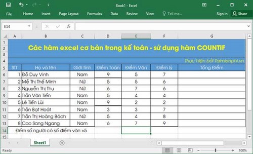
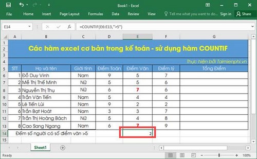
Example: Given a list of 8 students in a class, count the number of students whose Literature score is greater than 5.

The problem asks to use the COUNTIF function to calculate the number of students with a score >5, which is very easy. Apply the COUNTIF function to the following spreadsheet and work with TipsMake.

Applying the formula to the example above, the result allows us to select any cell, as in the example, E14 . Enter the formula as follows : =COUNTIF(E6:E13,'>5') where E6:E3 is the column of literature scores from number 1 to 8 with the filtering condition being >5.

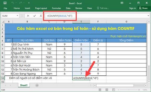
The result returned is 2. Upon checking, we can see that the table only contains 2 cases with a Literature score greater than 5.

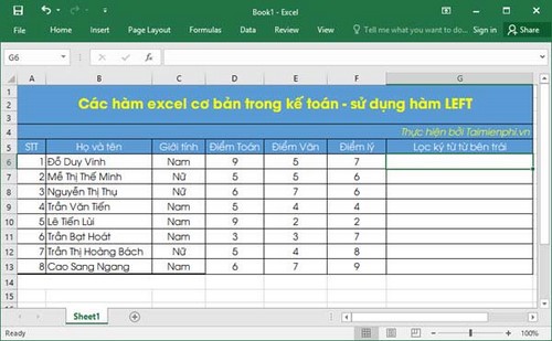
The LEFT function filters characters from the left side of a string.

The LEFT function filters values ​​from the left, extracting n characters from a referenced value. Using the LEFT function for searching and its reverse, as well as the RIGHT function, is very simple, as these are basic accounting functions, suitable for those new to Excel.

Syntax: =LEFT(text,[num_chars])

Text: The string of characters, rows, and columns from which to extract characters.
Num_chars: The condition applied to the string to be evaluated.

Explanation: The number of characters displayed will be counted from the left side and will depend on the value of Num_chars. The maximum number of characters displayed will be the total number of characters in that column or row.

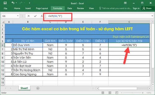
Example: Given a list of 8 students in a class, filter 5 characters so that the first number is ' Do Duy Vinh '.

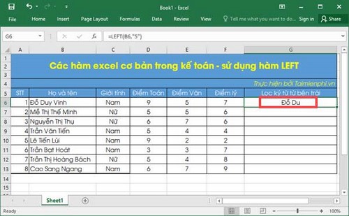
So the formula we enter here will be =LEFT(B6,'5') where B6 corresponds to the first number in the Full Name column, which is Do Duy Vinh, and we take 5 characters from the left.

The result we will get from 'Đỗ Du' will include spaces as well.

Although the above is just a simple way to use the LEFT function, there are many more uses of the LEFT function that you can discover after learning basic Excel functions in accounting.

VLOOKUP function – a search function

The VLOOKUP function in Excel helps you find and retrieve data from a specific string in a spreadsheet, which could be a student ID, employee ID, or product code, as required by the problem. Using the VLOOKUP function is slightly more difficult than the four functions above, but once you understand its nature, you'll find it extremely useful.

Syntax: =VLOOKUP(lookup_value,table_array,col_index_num,[range_lookup])

Lookup_value: The value used for searching.
Table_array: The table of values ​​to search in absolute address format (with a $ sign in front by pressing F4).
Col_index_num: The column order to retrieve from the lookup table.
Range_lookup: The search range, relative or absolute, with TRUE=1 (relative) and FALSE=0 (absolute).

Explanation: The VLOOKUP function is used to find values ​​for a row or column, depending on the problem requirements, with approximate (relative) or exact (absolute) values ​​if the conditions in the lookup table are met. VLOOKUP can also be used to reference values ​​in different tables.

Example: Given a list of 8 students in a class with different average scores, based on the Grading Rules table , display the results corresponding to the scores that each student achieved.

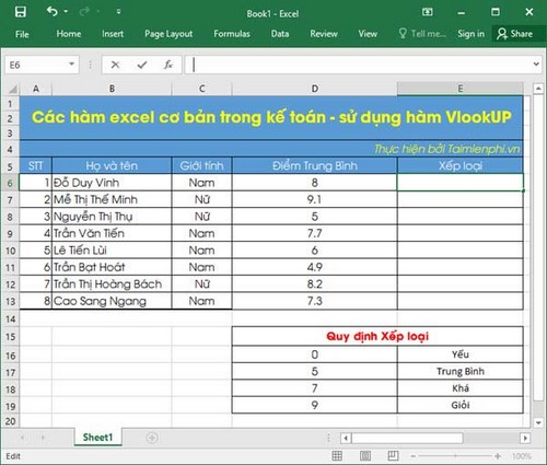
Based on the example above, we can understand that to return the result in column E (ranking), we first need to reference the average score column in the ranking table to find the corresponding result.

Therefore, the input syntax is as follows : =VLOOKUP(D6,$D$16:E$19,2,1) where D6 is the first position of the score column. $D$16:E$19 is the lookup table from position D16 to E19, and press F4 to display the $ before it. 2 is the column to be displayed in the second position, i.e., the text column, and 1 is the relative lookup value.

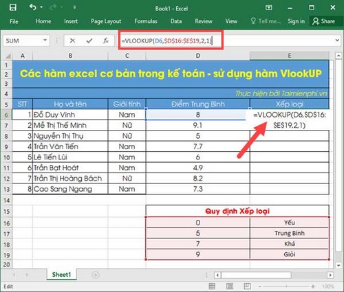
The displayed result in the relative search value will correspond to the values ​​in the established classification table, provided that the condition is met and the value is greater than or equal to the specified value.

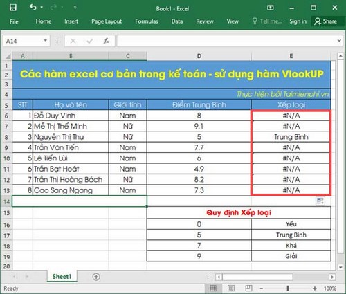
Alternatively, if you want to search by absolute value, you can enter =VLOOKUP(D6,$D$16:E$19,2,0) to get more precise results. However, please note that for lists requiring relative results, as in the example, searching by absolute value is unnecessary and the results will not be accurate as shown below.

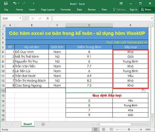
Using either relative or absolute values ​​has its own advantages. When we need the most precise result, absolute values ​​should be used. For results that allow for approximation or equivalence, relative values ​​will provide a more accurate representation.

Above, TipsMake has introduced you to 5 basic functions commonly used in accounting. These basic Excel functions will serve as a foundation for beginners and allow you to later learn more advanced functions. Furthermore, these basic Excel functions can be combined to create command sequences according to any requirements, producing the most satisfactory results.