How to create a Pivot Table in Google Sheets

The steps to create a Pivot Table in Google Sheets and Excel are slightly different. In fact, creating a Pivot Table in Google Sheets is more complex and difficult.

Instructions on creating a Pivot Table in Google Sheets

 

1. What is a Pivot Table?

As TipsMake mentioned above, Pivot Tables are designed to analyze and summarize large volumes of data, giving users a visual overview and enabling them to grasp spreadsheet data more quickly.

 

2. How to create a Pivot Table in Google Sheets

To create a Pivot Table in Google Sheets, follow these steps:

First, open the spreadsheet containing the data you want to use to create the Pivot Table in Google Sheets.

On the spreadsheet, select the cells you want to use in the Pivot Table. If you select the entire spreadsheet, you can skip this step.

Note: Each selected column must have a linked header to create a Pivot Table with those data points.

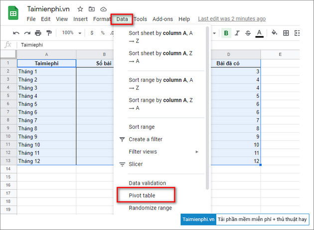
Next, on the Google Sheets menu bar, find and click Data => Pivot Table.

At this point, the Pivot Table creation window will appear on the screen. Here, in the Insert to section, you can select New Sheet to insert the table in a new sheet or Existing Sheet to insert the table in the current sheet.

If you select the Existing Sheet option , you will need to take an additional step to choose the location to add the sheet.

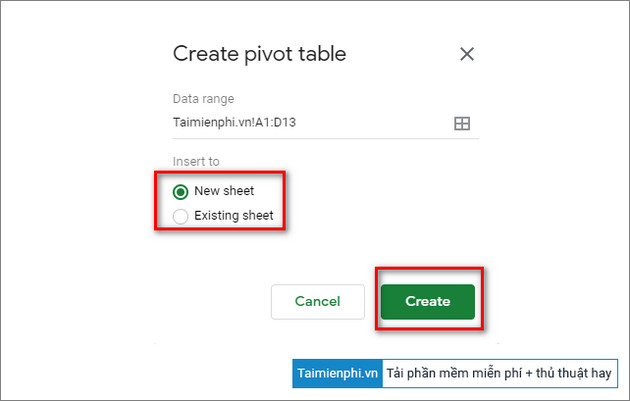
Once complete, click the Create button to generate a new Pivot Table.

Note: If the new statistics table does not open automatically, click on the Pivot Table located in the bottom corner of the spreadsheet.

 

Creating a bar chart in Google Sheets to compare data is a task many people need to perform, and the steps are quite simple, as outlined in this article.

 

3. Editing Pivot Tables in Google Sheets

On the Pivot Table window, on the right side you will see the table editing window. Here you will find options to add rows, columns, values, and filter data.

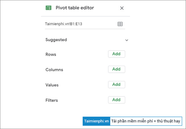
Select any option from the Suggested list and click the Add button next to it. Google Sheets will automatically create your summary table using the option you selected from the list.

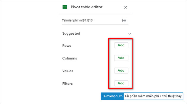
To customize the Pivot Table to your liking, click the Add button next to any option. In that section:

Rows option : adds all unique items of a specific column from the dataset to the Pivot Table as row headers. Columns
option : adds selected data points (headers) as aggregates to each column in the table. Values ​​option : adds the actual values ​​of each data point (or header) from the dataset so you can sort in the Pivot Table. Filter option : adds a filter to the table to display only data points that meet specific criteria.

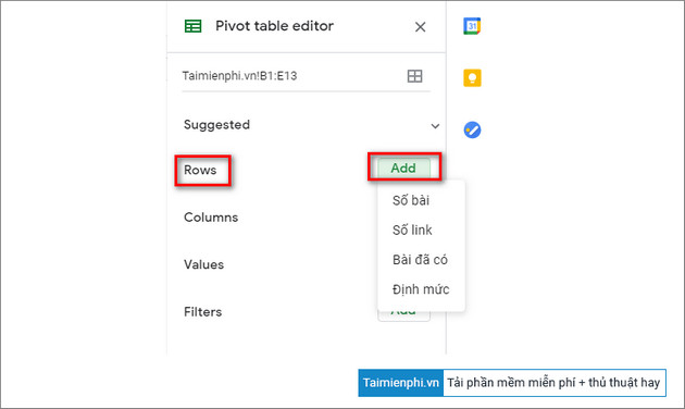
Click the Add button next to the Rows option and add the rows you want to display in the Pivot Table as shown below:

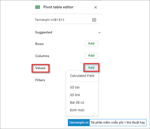
Next, click the Add button next to the Values ​​option and insert the values ​​you want to sort.

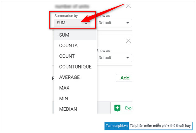
To change the values, click the dropdown menu icon in the Summarize by section and select any option including SUM, COUNT, AVERAGE, MIN, MAX, . .

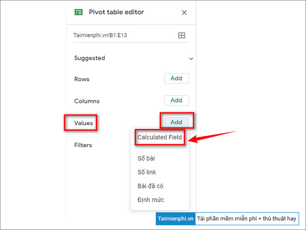
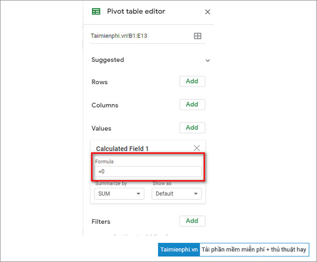
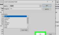
Additionally, if you wish, you can create your own formula by clicking the Add button next to the Values ​​option and selecting Calculated Field .

Enter any formula you wish to use in the box under the Formula section :

Finally, to add a filter to the table, click the Add button next to the Filters option .

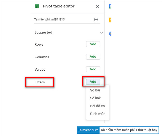
When adding a filter, you can select or deselect the values ​​you want to display on your table, then click OK to apply the changes.

Above, TipsMake has guided you on how to create a Pivot Table in Google Sheets. We wish you success.