3 Functions to Help You Stop Wasting Time in Excel

Most people think that speed in Excel means memorizing hundreds of formulas and functions. That's not the case until you discover that just 3 functions can replace the tons of formulas you used to struggle with.

3. XLOOKUP

Remember when VLOOKUP made you count columns just to find the column index? Or when you wanted to look up data to the left of the main column and ended up having to re-sort the entire spreadsheet? Those hassles are gone.

XLOOKUP is Excel's modern solution to all the flaws that VLOOKUP has. It's simpler and more flexible, and it's available in Excel 365 and Excel 2021+. Instead of struggling with column numbers or direction restrictions, you just tell it three things: What to look for, where to look for it, and what to return.

Here is the basic syntax:

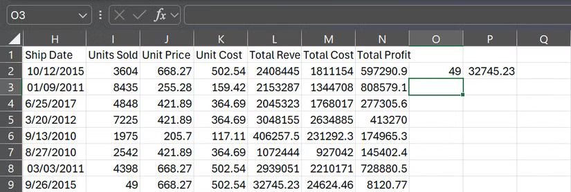
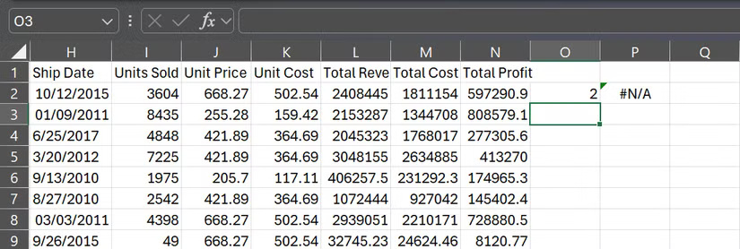
=XLOOKUP(lookup_value, lookup_array, return_array) =XLOOKUP(O2,I2:I200,L2:L200)

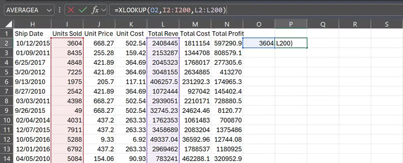
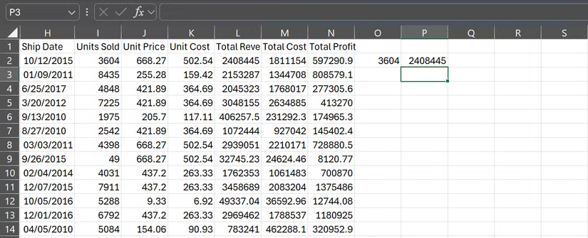
That's enough to look up a value and return a match. When you want to look up a different value, you don't need to change the cell specified as the lookup value (in our case, O2) in the formula. You just need to change the value in the cell (in our case, 3604) and the result will be updated immediately. If Excel doesn't find a match, it will display #N/A by default .

But XLOOKUP has some more useful tricks up its sleeve.

2. SUMIFS / COUNTIFS

If you're filtering your data every time you need to sum or count quickly, you're working too hard. SUMIFS and COUNTIFS are unsung heroes, especially for sales reports, budgets, or any data set that requires conditional calculations.

Imagine your boss asks you, "What is our total sales in Asia for products over $150 ordered online?" Instead of creating three filters and hoping not to break the spreadsheet, you can answer with one line:

=SUMIFS(sum_range, criteria_range1, criteria1, [criteria_range2, criteria2].) =SUMIFS(Sales_column,Region_column,"Asia",Price_column,">150",SalesChannel_column,"Online")

Or, in a real data set:

=SUMIFS(L2:L200,A2:A200,"Asia",J2:J200,">150",D2:D200,"Online")

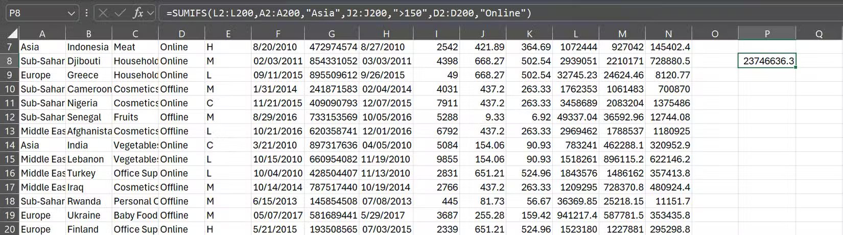
This formula sums all values ​​in column L, where column A equals "Asia", column J is greater than 150, and column D equals "Online".

Note : Make sure your criteria is enclosed in quotes if you are checking text values.

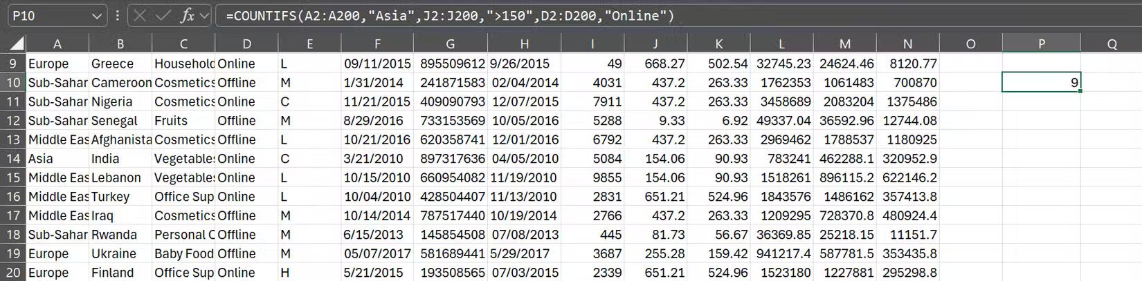
COUNTIFS works in a similar way, except it returns the number of rows that meet your conditions:

=COUNTIFS(criteria_range1, criteria1, [criteria_range2, criteria2].) =COUNTIFS(A2:A200,"Asia",J2:J200,">150",D2:D200,"Online")

Instead of the amount in SUMIFS, you will get the number of orders from Asia that were placed online and had a unit price over 150 USD.

SUMIFS and COUNTIFS also handle wildcards. For example, you can count all countries that start with the letter "T" and all items except fruit:

=COUNTIFS(B2:B200,"=A*",C2:C200, "Fruits")

Wildcards are handy, but they depend on clean data. If your data set has inconsistent capitalization or hidden characters, your results may be erroneous. A quick cleanup of your messy Excel spreadsheet will save you trouble later.

1. FILTER

The FILTER function might be the most satisfying function Excel has added in years. Remember when filtering data meant clicking through menus, setting conditions, and hoping you didn't accidentally hide the wrong row? With FILTER, all of that is reduced to a single formula, and the basic syntax is simple:

=FILTER(phạm vi cần lọc, tiêu chí lọc)

Let's say you want to see revenue from orders over $600:

=FILTER(Revenue_column,UnitsSold_column>600)

Or, in a real data set:

=FILTER(L2:L200,J2:J200>=600)

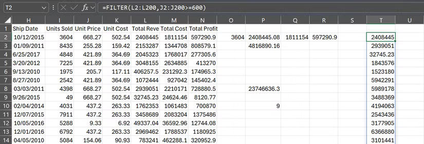
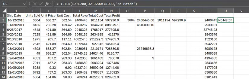
Right away, you'll see only numbers that match your criteria. If no values ​​match, you can also add a fallback message instead of getting an error:

=FILTER(L2:L200,J2:J200>=600)

Just like SUMIFS, you are not limited to one condition. You can use OR logic (at least one condition must be true) or AND logic (all conditions must be true). Here are some simple examples:

=FILTER(L2:L200,(J2:J200>=600)+(D2:D200="Online"),"No Match") =FILTER(L2:L200,(J2:J200>=600)*(D2:D200="Online"),"No Match")

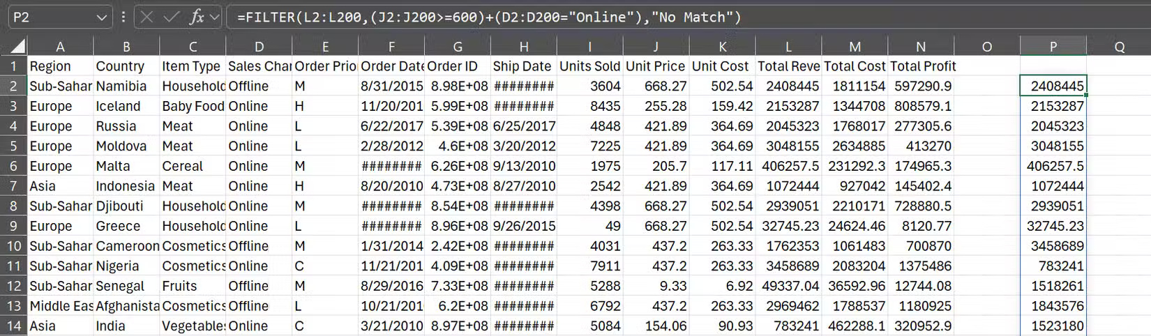
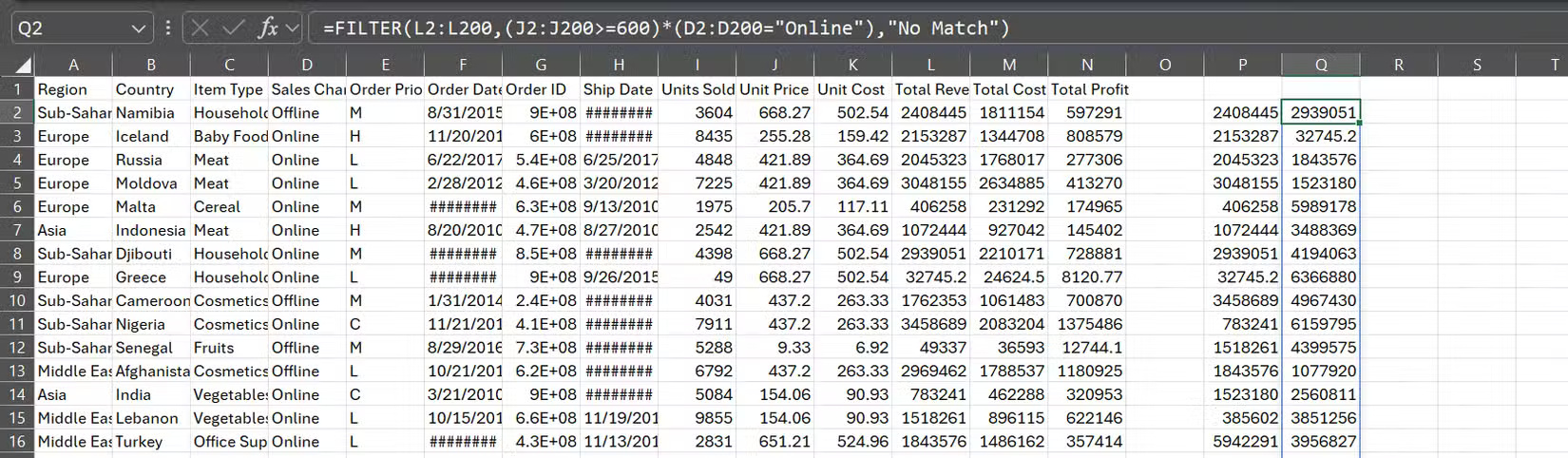
The first formula returns values ​​that cost over $600 or are sold online. The second formula returns only values ​​that cost over $600 and are sold online.

Tip : When using multiple conditions, enclose each condition in parentheses. Otherwise, Excel won't know how to evaluate them correctly.

FILTER is more efficient when combined with SORT. Let's say cell O2 contains "Meat" and you want to sort all matching rows by country:

=SORT(FILTER(A2:N200,C2:C200=O2,""),2,1)

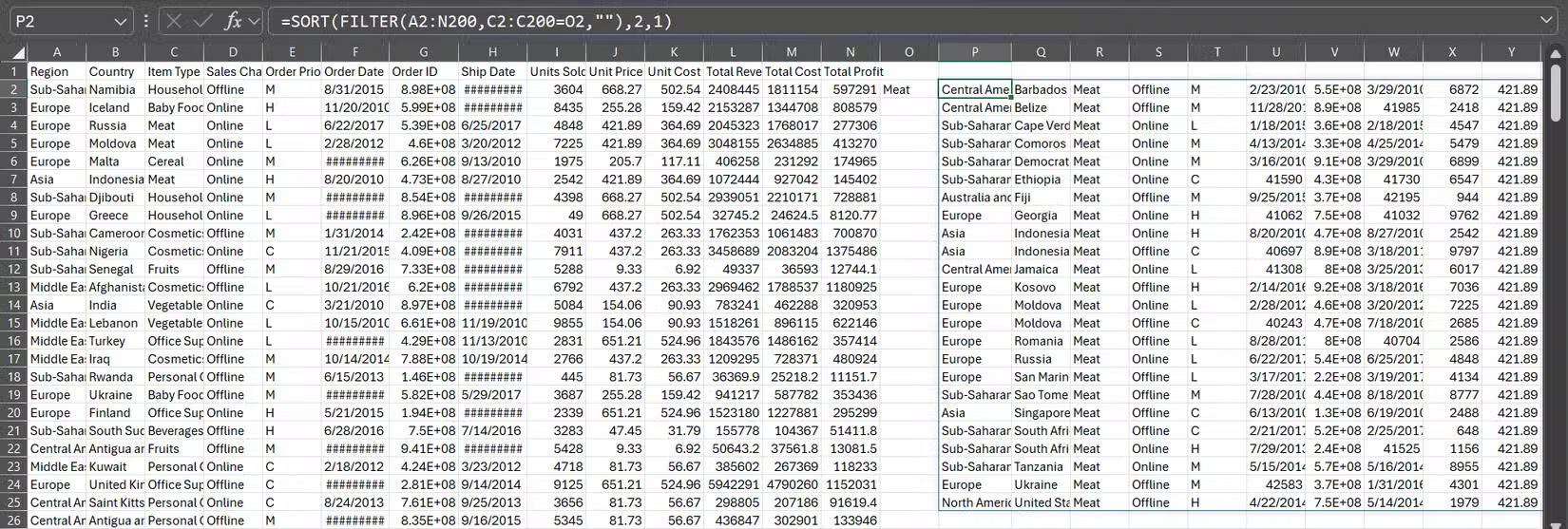
This gives you all the sales records for meat, sorted in ascending order by a specified column (in the example case, select column 2, i.e. the country column). Change the 1 at the end of the formula to -1, and your results will appear in descending order.

Kareem Winters

Update 25 August 2025