How to use the VLOOKUP function in Excel: formulas and detailed examples.

 

If you're new to  Excel , working with data can feel daunting. Let's explore how to use the VLOOKUP function to improve your skills.

What is Vlookup? Calculation formula and illustrative examples.

 

Quick Overview:
I. What is the Vlookup function?
II. Syntax
III. Illustrative Examples
IV. How to combine Vlookup with Hlookup, Left, Right, and Match
V. Common Errors When Using the Function

I. What is the VLOOKUP function?

VLOOKUP is a basic and common function in Excel that allows users to search for data by column. You can quickly look up and get the desired results with just a few clicks.
 

II. Usage Syntax

In there:

- lookup_value: The value used for searching.

-  table_array: The lookup table, set to Absolute address format (with a $ sign in front by pressing F4).

-  col_index_num: The order of the column from which to retrieve data in the lookup table.

-  range_lookup: The search range. TRUE is equivalent to 1 (relative lookup), FALSE is equivalent to 0 (absolute lookup).
 

III. Illustrative Examples

With Vlookup's relative and absolute lookup capabilities, you can easily summarize data in Excel spreadsheets, helping you to compile details for reports, filter out necessary lists, and make your work more accurate and time-efficient.
 

1. Relative search

Example: Based on the grading scale corresponding to the given scores, determine the academic performance of the students listed below:

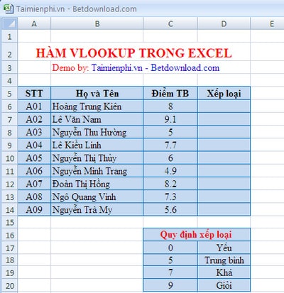
Example of the Vlookup function in Excel

We use the formula in column D6: =VLOOKUP(C6,$C$16:$D$20,2,1)
The result obtained is:

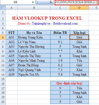
Results when using the VLOOKUP function
 

2. Absolute search

Using an absolute search will yield more detailed results than a relative search.
For example: Fill in the information on the hometown and qualifications of employees in the table based on the corresponding employee codes below.

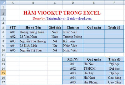
Example of absolute lookup using the VLOOKUP function.

To fill in the employee's hometown information, use the VLOOKUP formula in cell E6 as follows: =VLOOKUP(A6,$D$12:$F$17,2,0)
A6 is the value to look up
$D$12:$F$17 is the lookup table
2 : column number in the lookup table
0 : Exact match type

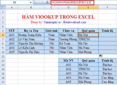
Similarly, to fill in the employee's qualification field, do the following:

The formula for cell F6 is: =VLOOKUP(A6,$D$12:$F$17,3,0)

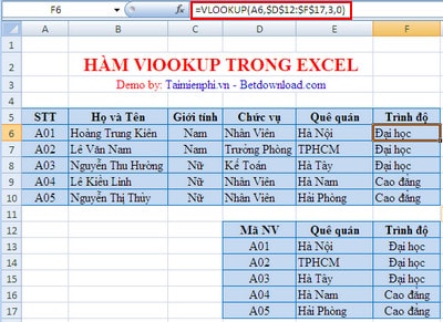
Results when searching for absolute value

3. Relative value and absolute value

Using absolute values ​​will give you the most accurate results. Absolute values ​​will not change their addresses even if they appear in new columns or cells. Therefore, we use absolute values ​​when we need to find the most precise information and relative values ​​when we need to find the most accurate or nearly accurate results. To learn more, you can refer to the article on referencing functions in Excel .

 

IV. How to combine Vlookup with Hlookup, Left, Right, and Match

This problem combines lookup functions with Hlookup functions , or Left, Right, and Match functions.

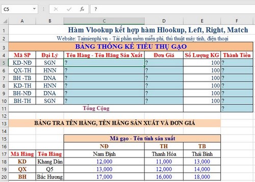
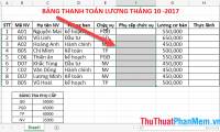
Given the data as shown in the table below, with the following conventions:
- Table 1: RICE CONSUMPTION STATISTICS
- Table 2: TABLE OF PRODUCT NAMES, MANUFACTURER NAMES AND UNIT PRICES

The following needs to be addressed:

Question 1: Based on the two left and two right characters of the Product Code in Table 1, look up the values ​​in Table 2 to fill in the Product Name - Manufacturer Name column (Calculate data for columns C5:C10).
Example: KD-ND means Khang Dan rice - Nam Dinh.
Question 2: Fill in the Unit Price for each item based on the Product Code in Table 1 and look it up in Table 2. (Calculate data for columns D5:D10).
Question 3: Calculate the total amount = Quantity * Unit Price

Answer:

Question 1:
- Explanation: We need to provide a formula to retrieve the Product Name and the Province of Manufacture data, then combine these two formulas to get the answer to Question 1.

 + Get Product Name: Take the leftmost 2 characters in the Product Code column in Table 1 (A5:A10) and compare them to the 2 characters in the Product Code column in Table 2, but the data range should also include the Product Name column in Table 2 (A15:B20) or (A15:E20).
 >> We use the VLOOKUP function: In a cell that doesn't have data, try entering the following formula: =VLOOKUP(LEFT(A5,2),$A$15:$B$20,2,FALSE)
After entering, press Enter. If the word "Khang Dân" appears, you've completed 40% of the answer to Question 1. Simple, right? Let's continue.

+ Get the Province Name of Production: Compare the two characters on the right in the Product Code column (A5:A10) in Table 1 with the two characters in the "Row" Rice Code - Province Name of Production in Table 2. The data range to be retrieved will be (A16:E20).
 >> To retrieve data by row, we use the Hlookup function. In a cell that doesn't have data, try entering the following formula:

= HLOOKUP(RIGHT(A5,2),$C$16:$E$20,2,FALSE)
After entering the code, press Enter again. If the result is "Nam Dinh", you have completed 40% of the answer to Question 1. At this point, you should have a good idea of ​​the answer, right? The next step is to combine these two functions to calculate the data in the Product Name - Province Name column.

+ Combining two formulas: There are many formulas to combine or concatenate strings together. In this problem, Free Download guides you on how to concatenate strings using the & function. In this problem, we will use a hyphen (with a space) to separate the two formulas that have already calculated the results, namely the Product Name and the Province of Production Name, specifically: " - "
 In summary, the function will be as follows: =+vlookup&" - "&hlookup (No equals sign at the beginning of the Hlookup function anymore).
 Then, in cell C5, enter the formula:
 C5=+VLOOKUP(LEFT(A5,2),$A$15:$B$20,2,FALSE)&" - "&HLOOKUP(RIGHT(A5,2),$C$16:$E$20,2,FALSE)
 Press Enter to see the result. If the answer is correct, it should be "Khang Dan - Nam Dinh".
 Once the result is correct, in the next cell C6:C10, just point your mouse to the formula in cell C5 and drag it down to C10, and you're done
 . Similarly,

C6=+VLOOKUP(LEFT(A6,2),$A$15:$B$20,2,FALSE)&" - "&HLOOKUP(RIGHT(A6,2),$C$16:$E$20,2,FALSE)
That completes Question 1 of the problem. Let's continue to solve Question 2.

Question 2: Calculate the
Unit Price. The formula will be as follows: In cell D5, enter the formula
D5=+VLOOKUP(LEFT(A5,2),$A$16:$E$20,MATCH(RIGHT(A5,2),$A$16:$E$16,0),FALSE)

Question 3: Calculate the total amount.
Oh, this question often appears in data calculation problems such as payroll, expenses, total amount, etc. It's quite easy, isn't it?
The formula for calculating the total amount is as follows: In cell F5, enter E5 = + D5 * E5

 

V. Common errors when using

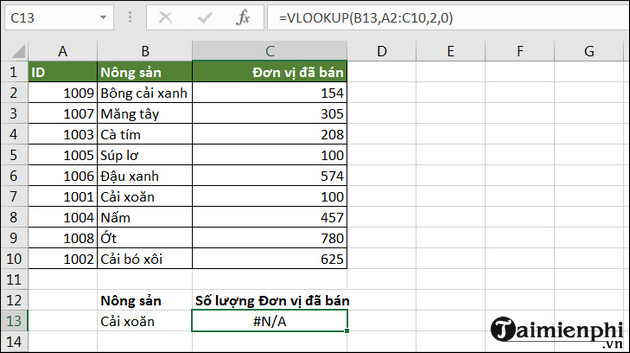
1. Error #N/A

What is the #NA error?  The #NA error is returned in an Excel formula when a suitable value is not found. When using VLOOKUP, we encounter the #NA error when the search condition is not found in the control, specifically in the first column of the function's condition range.

 

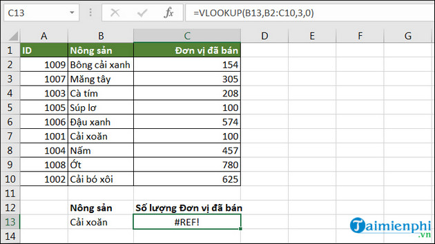
2. Error #REF!

The #REF! error occurs when the specified column is undefined, for example, in the example below,  Col_index_num is 3 , while Table_array is B2:C10, which only has 2 columns. Therefore, the system will report the #REF! error.

 

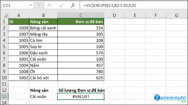
3. Error #VALUE!

The #VALUE! error occurs when the  Col_index_num column in the formula is less than 1. For example, in the example below,  Col_index_num equals 0 , resulting in the #VALUE! error.

 

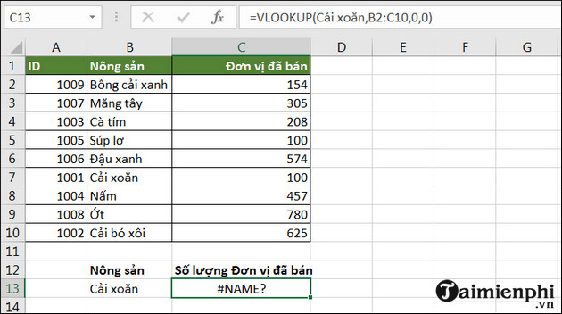
4. Error #NAME?

The #NAME? error  appears when Lookup_value is missing quotation marks ("") (quotation marks are used to format text and help Excel understand formulas). For example, the example below shows " Cabbage " but it lacks quotation marks (""), causing Excel to misunderstand the formula.  To fix this, replace " Cabbage " with "Cabbage" .

 

VI. Some notes when using the VLOOKUP function

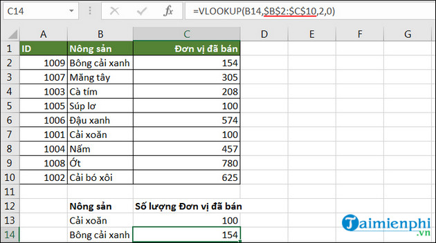
1. Use absolute references

Using absolute references allows you to copy formulas from one column to another without them changing.

As in the example below, the formula in cell C13 is =VLOOKUP(B13,$B$2:$C$10,2,0) . When copying this formula to cell C14, Table_array will remain unchanged.

 

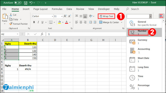
2. Do not save numerical values ​​as text.

If the numerical data in the data table is in text format, as in the example below for column A, when you enter the formula =VLOOKUP(A8$A$2:$B$5,2,0) in the revenue column, the data will return the #N/A error. To convert text data to numbers, simply select Home => Select Wrap Text => Select Number .

 

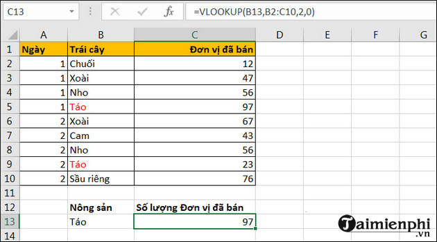
3. The lookup table contains duplicate values.

If your table contains multiple duplicate values, the VLOOKUP function will return the first result it finds from top to bottom. For example, in the table, it returns the result "Apple" as 97 instead of 23 below.

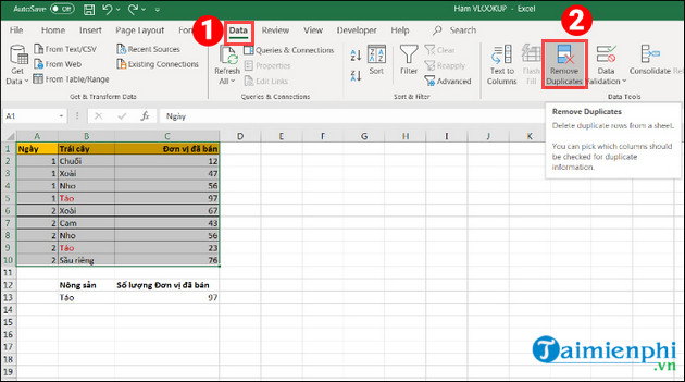
Solution 1: If you want to remove duplicate values, highlight the lookup table and select Data  => Select  Remove Duplicates

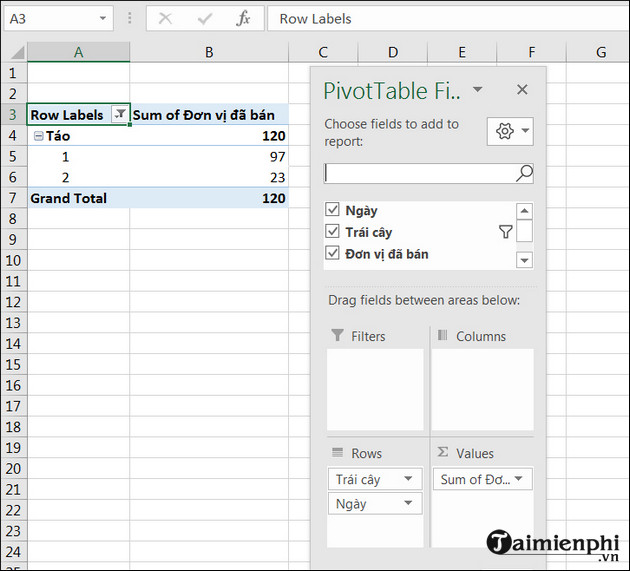
Solution 2: Use a Pivot Table to filter the results list.

The VLOOKUP function in Excel helps you look up and return matching values ​​from a data table, supporting quick column-based searches. This function has two modes: relative lookup for approximate values ​​and absolute lookup for exact matches. To improve lookup efficiency, you can combine VLOOKUP with MATCH for more flexibility in identifying the data column to retrieve results from. If you want to look up rows instead of columns, the HLOOKUP function is a suitable choice. Understanding how these functions work and combining them flexibly will help you process data more quickly and accurately in Excel.