10 EXCEL functions that ACCOUNTERS often use

Using excel and functions in excel is one of the basic skills that accountants must be proficient. In Excel, there are many functions that can help accountants in daily data entry, but here are some of the most commonly used accounting functions.

1. SUMMER, AVERAGE

10 EXCEL functions that ACCOUNTERS often use Picture 1

SUMMER, AVERAGE

1. Syntax: = SUM (number 1, number 2, ., number or range of data)

Meaning: A function to sum values

For example: = SUM (4,5,1) => Result = 10

1. Syntax: = AVERAGE (value 1, value 2, value 3, . value n or data range)

Meaning: A function that returns the average of the parameters entered or of a data area

For example: = SUM (7,8,9) => Result = 8

2. SEARCH (VLOOKUP)

1. V stands for Vertical meaning vertical (vertical). Lookup is a reference and search function

VLOOKUP means search vertically, by column

1. Syntax: = VLOOKUP (x, reference region, nth column, 0)

Meaning: take a value (x) to compare by the column of the reference region to return the value in the corresponding column in the reference area (the nth column), 0: compare the dark, 1: absolute comparison dark

Attention:

1. Reference region: the first column of the reference must cover only the entire search values ​​adequately.Always have to be at absolute value
2. The column to count counts as to how much it is in the reference table.When counting must count from left to right

3. FUNCTION IF

1. Syntax: = If (Logical_test, [value_if_true], [value_if_false]) means If (Condition, value 1, value 2)

Meaning: A function that returns value 1 if the condition is true, the function returns value 2 if the condition is false

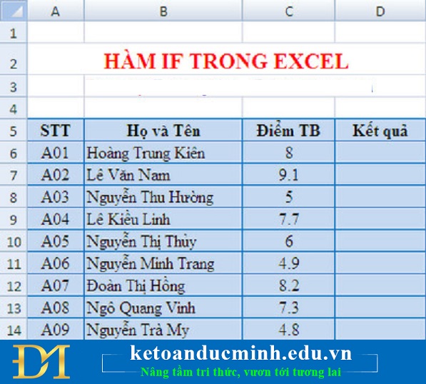
Example: Given a student's transcript, review the results to see if the student passed or had to retake the test

With the following data sheet:

Average score> = 5: Do

Medium score

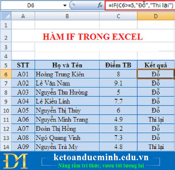
We use the formula for cell D6 as: = IF (C6> = 5, "Do", "Retake")

10 EXCEL functions that ACCOUNTERS often use Picture 2

FUNCTION IF

You have got the results of students passing or retesting

10 EXCEL functions that ACCOUNTERS often use Picture 3

FUNCTION IF

4. SUMIF

1. Syntax: = SUMIF ((range, criteria, sum_range) means Sumif (Conditional container, conditional, sum area)

Meaning: This function returns the sum of the cells in the range to satisfy a given condition

Attention:

1. Due to calculations in Excel cells, SUMIF function sums on Excel 2016, Excel 2013, or earlier versions like Excel 2010, 2007, 2003 applying the same function structure.

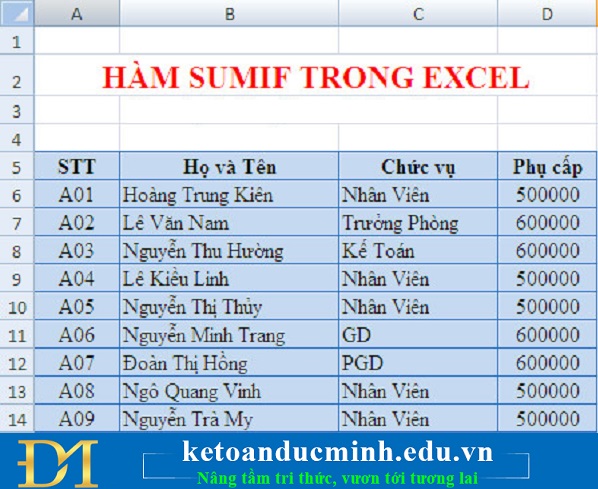
For example: The problem of using SumIF function to calculate the allowances for those who have the position of "Staff" in the table below:

10 EXCEL functions that ACCOUNTERS often use Picture 4

SUMIF

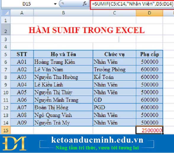
With the formula for cell D15 is: = SUMIF (C5: C14, "Staff", D5: D14)

10 EXCEL functions that ACCOUNTERS often use Picture 5

SUMIF

We get the following result: 2500000. When we check the results, we find that in the VD Sumif function there are 5 people with the position of "Staff", so the total allowance for those people with the result is 2500000 is correct.

5. AND AND OR

1. Syntax: = AND ((Logical1; [Logical2]; [Logical3]; .) means And (against 1, against 2, .)

Meaning: This function is AND AND, true only when all arguments are true.The arguments are constants, logical expressions

Attention:

1. The AND function has up to 256 arguments that must be logical values ​​or arrays or references that contain logical values.All values ​​will be ignored if an array or reference argument contains text or empty cells.
2. The arguments must be either logical values ​​or arrays that contain logical values.
3. If the reference arguments are text values ​​or null (null) then those values ​​are ignored.
4. If the reference range does not contain a logical value, the function returns the #VALUE! Error.

Example 1: Use the AND function to know if the following formulas are true or false.

Browse students' names and genders right or wrong

With the formula in C6: = AND (A6 = "Nguyen Van Dat", B6 = "Nam")

10 EXCEL functions that ACCOUNTERS often use Picture 6

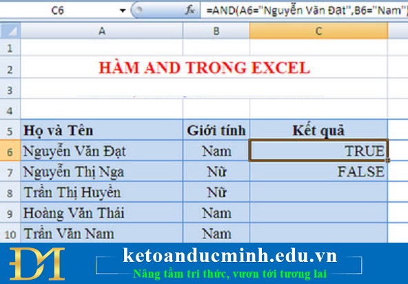
AND FUNCTION

If true, the result will be TRUE

10 EXCEL functions that ACCOUNTERS often use Picture 7

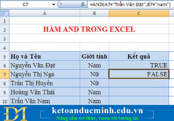
AND FUNCTION

Otherwise, you will get FALSE

1. Syntax: = OR (((Logical1; [Logical2]; [Logical3]; .) means Or (against 1, against 2, .)

Meaning: This function is OR OR, false only when all arguments are false

For example: = OR (F7> February 3, 76, F7> January 1, 2016)

6. COUNTIF

10 EXCEL functions that ACCOUNTERS often use Picture 8

COUNTIF

1. Syntax: = COUNTIF (range, criteria)

Inside:

Range: is the data range that you want to count conditionally.

Criteria: the condition for a cell to be counted.

Meaning: The Excel COUNTIF function is used to count the number of cells that meet the criteria (Criteria) in the range (Range).

Example: = COUNTIF (B4: B1, '> 500 ″)

This means counting all the cells in the B4: B12 series that contain numbers greater than 500

7. MIN, MIN, MAX

10 EXCEL functions that ACCOUNTERS often use Picture 9

MINUTES MIN, MAX

1. Syntax: = MAX (number 1, number 2, .)

Meaning: Returns the maximum value of number1, number 2, . or the maximum value of a whole range of numeric data.

Example: MAX (10,20,30) = 30

1. Syntax: = MIN (number 1, number 2, .)

Meaning: Returns the smallest value of number1, number 2, . or the smallest value of a whole range of numeric data

Example: Min (10,20,30) = 10

8. FUNCTION LEFT, RIGHT

1. Syntax: = LEFT (string, character to be retrieved)

Meaning: To separate characters to the left of the string

For example: = LEFT ('THANH HUE', 4) => Result: = THANH

1. Syntax: = RIGHT (string, characters you want to retrieve)

Meaning: To separate characters to the right of the string

For example: = LEFT ('THANH HUE', 3) => Result: = HUE

9. SUBTOTAL FUNCTION

10 EXCEL functions that ACCOUNTERS often use Picture 10

FUNCTION SUBTOTAL

1. Syntax: = SUBTOTAL ((function_num, ref1, [ref2], .)

Inside:

1. Function_num: Required.Numbers 1-11 or 101-111 specify the function used for subtotals.1-11 include hidden rows manually, while 101-111 excludes them;Filtered cells will always be excluded.
2. Ref1 Required.The first named range or reference for which you want to subtotal.
3. Ref2, . Optional.The range or series is named from 2 to 254 that you want to subtotal for it.

Attention:

1. If there are other nested SUBTOTAL functions placed on ref1, ref2, etc., then these nested functions will not be counted to avoid double counting.
2. The Function_num argument, if from 1 to 11, the calculated SUBTOTAL function includes values ​​in the dataset (hidden rows).The Function_num argument is between 101 and 111, the SUBTOTAL function only calculates for non-hidden values ​​in the dataset (ignoring the hidden values).
3. The SUBTOTAL function will skip counting all rows hidden by the Filter (Auto Filter) command regardless of the Function_num argument used.
4. The SUBTOTAL function is designed to calculate vertical columns of data, it is not designed to be horizontal.
5. This function only calculates for 2-D data so if the reference data is in 3-D format then the SUBTOTAL function reports the #VALUE error.

10. HAm NOW

10 EXCEL functions that ACCOUNTERS often use Picture 11

HAM NOW

1. Syntax: = NOW ()

The NOW function syntax has no arguments

Meaning: The function = NOW () to display the system date and time in the calculation.For example:

You only need to enter the function = now () and press Enter will immediately display the date and time at the current time as shown below.

Attention:

1. There may be an error ####, but you just need to drag the cell a little wider and it will be OK