Complete financial functions in Excel you should know

In Excel, financial functions for calculating profits, calculating dates, or calculating time are essential in the workflow of almost all businesses. In this article, we will follow the usage of financial functions in the most detailed and easy to understand.

1. FV function

Use : Used to calculate the future value of an investment based on a fixed interest rate.

Formula : = FV (rate, nper, pmt, [pv], [type])

In which :

+ Rate (required): Interest rate by term.

+ Nper (required): Total number of payment terms.

+ Pmt (required): Payment for each period; This clause remains unchanged. Typically, pmt contains principal and interest, but no other fees and taxes. If pmt is omitted, you must include the pv argument.

+ Pv (optional): Present value, or present one-time payment equal to a series of future payments. If pv is omitted, it is assumed to be 0 and you must include the pmt argument.

+ Type (optional): Number 0 or 1 indicates when the payment is due. If type is omitted, it is assumed to be 0.

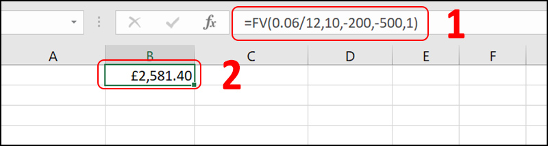
Example : Annual interest rate is 6%, total number of payments is 10, amount payable is 200, present value is 500, payment at the beginning of the period. Entering the formula = FV (0.06 / 12,10, -200, -500,1) (1) will give $ 2,581.40 (2).

Complete financial functions in Excel you should know Picture 1

2. The function creates the date

DATE function

Use : Returns a specified date.

Formula : = DATE (year, month, day)

Example : In the example we need to sum your dates of birth but currently the cells are separate, we use the DATE function to sum your dates. Year in cell D2, Month in cell C2, Day in cell B2. Entering the DATE formula (D2, C2, B2) (1) gives the result January 12, 2002 (2).

Complete financial functions in Excel you should know Picture 2

- DATEVALUE function

Usage : Converts a text string with the form of a date to a date value that can be calculated.

Formula : = DATEVALUE (date_text)

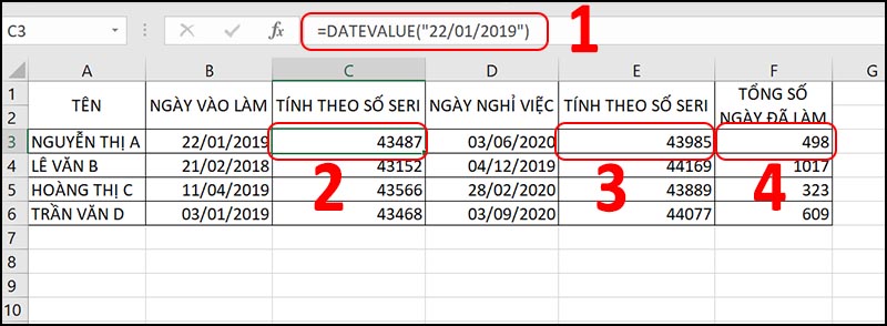
Example : Use the DATEVALUE function to convert dates to serial numbers, then subtract the days off from work and the number of days that employee worked will produce the result (4).

Complete financial functions in Excel you should know Picture 3

3. The current date and time functions

- TODAY function

Use : Returns the current date. Often TODAY is used to quickly calculate time.

Formula : = TODAY ()

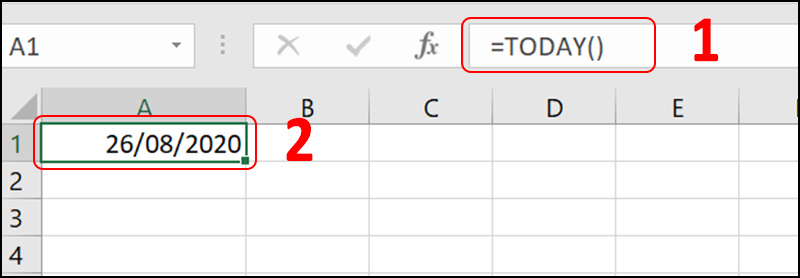
Example : Let's say today is August 26, 2020. Entering the formula = TODAY () (1) gives the result 08/26/2020 (2).

Complete financial functions in Excel you should know Picture 4

- Function NOW

Usage : Returns the current date and time.

Formula : = NOW ()

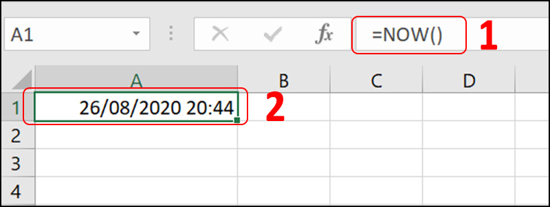
For example : Let's say the current time is 20:44 on 08/26/2020. Entering the formula = NOW () (1) will result (2).

Complete financial functions in Excel you should know Picture 5

4. The function extracts the date and date components

- DAY function

Use : Returns the day of the month.

Formula : = DAY (serial_number)

Of which : Serial_number (required): The date of the date you are trying to find. The dates should be entered by using the DATE function or as the results of other formulas or functions.

Example : Use DAY to quote a date in May 22, 2019. Entering the formula = DAY ('22 / 5/2019 ') (1) will return a 22 (2) result.

Complete financial functions in Excel you should know Picture 6

- MONTH function

Utility : Returns the month of the specified date.

Formula : = MONTH (serial_number)

Of which : Serial_number (required): The date of the month you are trying to find. Dates should be entered by using the DATE function or using the results of other formulas or functions.

Example : Using the MONTH function to quote the month from May 22, 2019, entering the formula = MONTH ('May 22, 2019') (1) will return May (2).

Complete financial functions in Excel you should know Picture 7

- YEAR function

Use : Returns the year of a given date.

Formula : = YEAR (serial_number)

Of which : Serial_number (required): The date of the month you are trying to find. Dates should be entered by using the DATE function or using the results of other formulas or functions.

Example : Use the YEAR function to extract the year from May 22, 2019. Entering the formula = YEAR ('22 / 5/2019 ') (1) will return 2019.

Complete financial functions in Excel you should know Picture 8

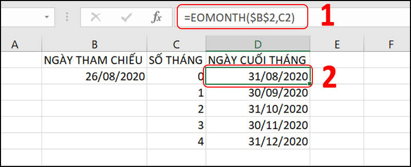
- EOMONTH function

Use : Returns the last day of the month.

Formula : = EOMONTH (start_date, months)

In which :

+ Start_date (required): Date represents the start date. Dates should be entered by using the DATE function or using the results of other formulas or functions.

+ Months (required): Number of months before or after start_date. A positive value for the months argument produces a future date; Negative values ​​create a date in the past.

Example : To know the last days of the months 8, 9, 10, 11, and 12 of 2020 we use the function EOMONTH . Start_date is August 26, 2020, which is B2. Months is the number of consecutive months since Start_date, in our example 0, 1, 2, 3, 4. When entering the formula = EOMONTH ($ B $ 2, C2) (1) the result is the last date. months of these months (2).

Complete financial functions in Excel you should know Picture 9

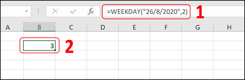
- WEEKDAY function

Use : Returns the day of the week corresponding to a date.

Formula : = WEEKDAY (serial_number, [return_type])

In which :

+ Serial_number (required): Is a serial number representing the date of the date you are looking for. Dates should be entered using the DATE function or entered as the results of other formulas or functions.

+ Return_type (optional): Is a number that defines the type of return value.

For example : When we need to know what day of the week, August 26, 2020, we use the WEEKDAY function . Where serial_number is 26/8/2020, return_type is 2 to calculate the time from Monday to Sunday. When entering the formula = WEEKDAY ('26 / 8/2020 ') the result is 3 i.e. 26/8/2020 (2) is the 3rd place date of the week, which is Wednesday.

Complete financial functions in Excel you should know Picture 10

- WEEKNUM function

Utility : Returns the number of the week of the year for a specified date.

Formula : = WEEKNUM (serial_number, [return_type])

In which :

+ Serial_number (required): Is a day of the week. Dates should be entered using the DATE function or entered as the results of other formulas or functions.

+ Return_type (optional): Is a number to specify which date the week will start. Default is 1.

For example : When we need to know what week is the week of August 26, 2020, we use the function WEEKNUM . Where serial_number is 26/8/2020, return_type is 2 to calculate the time from Monday. When entering the formula = WEEKNUM ('26 / 8/2020 ', 2) the result is 35, ie the week containing August 26, 2020 is the 35th week of the year.

Complete financial functions in Excel you should know Picture 11

5. Function to calculate the difference of the date

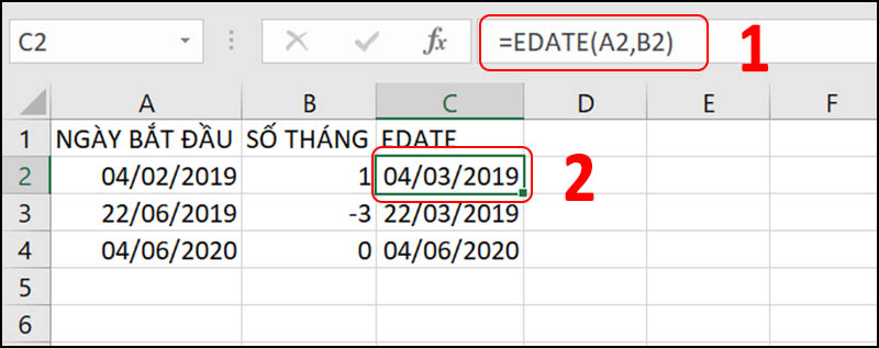
- EDATE function

Utility : Returns a date within the specified month that can be preceded or after the start date. Use the EDATE function to calculate due dates or due dates on the issue of the month.

Formula : EDATE (start_date, months)

In which :

+ Start_date (required) Date represents the start date. Dates should be entered by using the DATE function or using the results of other formulas or functions.

+ Months (required): Number of months before or after start_date. A positive value for the months argument produces a future date; Negative values ​​create a date in the past.

Example : To know what date the next month of February 4, 2019 is, use the EDATE function with Start_date as February 4, 2019, Months is 1. When entering the formula = EDATE (A2, B2) (1) will return March 4, 2019 (2).

Complete financial functions in Excel you should know Picture 12

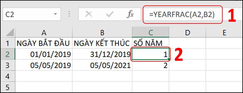
- YEARFRAC function

Usage : The YEARFRAC function calculates the part of the year represented by the number of whole days between two dates (start_date and end_date).

Formula : = YEARFRAC (start_date, end_date, [basis])

In which :

+ Start_date (required): Start date.

+ End_date (required): End date.

+ Basis (optional): Type of date basis to use.

For example , we use the YEARFRAC function to calculate how many years between December 31, 2019 and January 1, 2019. Star_date is January 1, 2019, End_date is December 31, 2019. Entering the formula = YEARFRAC (A2, B2) (1) will return 1 (2) because it is 1 year between these two periods.

Complete financial functions in Excel you should know Picture 13

6. Function to calculate working days

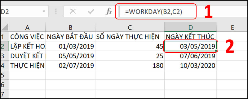
- Function WORKDAY

Utility : Returns a sequence number representing the number of workdays, either before or after the work start date, and subtracting weekends and holidays (if any) in that time period.

Formula : WORKDAY (Start_date, Days, [Holidays])

In which :

+ Start_date: Is the start date, is a required parameter.

+ Days: Is the date not in weekends and holidays before or after Start_date, is a required parameter.

Holidays: Days to be excluded from working days that are not a fixed holiday date.

Example : To perform quickly when determining the end date of a project, we will use the function WORKDAY . Start_date is March 1, 2019, days are 45 days, for example, working without holidays. Entering the formula = WORKDAY (B2, C2) (1) will return 5/5/2019 (2).

Complete financial functions in Excel you should know Picture 14

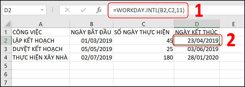
- Function WORKDAY.INTL

Usage : This is a function that returns a date before or after the start date by a specified number of business days with a custom weekend. Weekend parameters indicate which and how many days there are.

Formula : WORKDAY.INTL (start_date, days, [weekend], [holidays])

In which :

+ Start_date (required): Start date.

+ Days (required): Number of working days before or after start_date. A positive value results in a future date; Negative values ​​result in a date in the past; the value 0 returns start_date.

+ Weekend (optional): Indicates which days of the week are weekend days and are not considered working days. Weekend is a weekend number or string that specifies when a weekend occurs.

For example : We need to specify the start date and the end date of the job with specifying the weekend as you want, we will use the function WORKDAY.INLT . Start_date is March 1, 2019, days are 45 days, Weekend is Sunday by default. When you enter the formula = WORKDAY.INTL (B2, C2,11) (1) will give the result. is April 23, 2019 (2).

Complete financial functions in Excel you should know Picture 15

- NETWORKDAYS function

Usage : Returns the number of full working days from start_date to end_date. Working days do not include weekends and any public holidays specified. Use the NETWORKDAYS function to calculate employee benefits accrued based on the number of days worked in a specific period.

Formula : = NETWORKDAYS (start_date, end_date, [holidays])

In which :

+ Start_date (required): Start date.

+ End_date (required): End date.

Holidays (optional): An optional range of one or more days to be excluded from the business calendar, such as federal holidays, state holidays and non-fixed holidays.

Example : Use the NETWORKDAYS function to calculate the number of workdays. Start_date is March 1, 2019, End_date is April 2, 2019. Entering the formula = NETWORKDAY (B2, C2) (1) will yield 23 (2), which takes 23 days to plan. Note, Excel does not work Saturdays and Sundays by default.

Complete financial functions in Excel you should know Picture 16

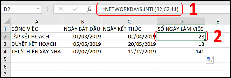
- NETWORKDAYS.INTL function

Usage : Returns the number of full workdays between two dates by using parameters to indicate how many weekends there are and which ones. Weekends and any days specified as public holidays are not considered business days.

Formula : = NETWORKDAYS.INTL (start_date, end_date, [weekend], [holidays])

In which :

+ Start_date and end_date (required): The days need to calculate the distance between them. Start_date can be earlier, the same as or later than end_date.

+ Weekend (optional): Indicates which days are weekends and are not counted towards the number of full working days from start_date to end_date. Weekends can be the number of weekends or a string indicating when weekends occurred.

Example : Using the NETWORKDAYS.INTL function to calculate the number of working days, determine the weekend day as you want. Start_date is March 1, 2019, End_date is April 2, 2019, Weekend is Sunday by default 11. When entering the formula = NETWORKDAYS.INTL (B2, C2,11) (1) will give It returns 28 (2), which takes 23 days to plan.

Complete financial functions in Excel you should know Picture 17

7. Time functions in Excel

- TIME function

Use : Returns the time as a serial number.

Formula : = TIME (hour, minute, second)

In which :

+ Hour (required): Is a number from 0 to 32767 representing hours. Any values ​​greater than 23 will be divided by 24 and the remainder will be considered the hour values.

+ Minute (required): Is a number from 0 to 32767 representing minutes. Any value greater than 59 will be converted to hours and minutes.

+ Second (required): Is a number from 0 to 32767 representing seconds. Any value greater than 59 will be converted to hours, minutes, and seconds.

Example : To specify 9:46 AM we enter Time as 9, Minute is 45, Second is 34. When entering the formula TIME (0,45,34) (1) will give 9:45 AM (2 ).

Complete financial functions in Excel you should know Picture 18

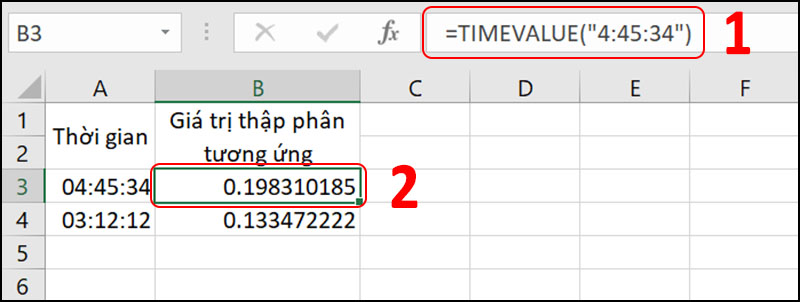
- TIMEVALUE function

Usage : Returns the decimal number of the time represented by a text string.

Formula : = TIMEVALUE (time_text)

Of which : Time_text (required): Is a text string representing time in one of Microsoft Excel's time formats; for example, the text strings "6:45 PM" and "18:45" are enclosed in quotation marks representing the time.

For example : When you need to find the corresponding decimal value of 4:45:34, enter the formula = TIMEVALUE ('4:45:34') (1) will give 0.198310185 (2).

Complete financial functions in Excel you should know Picture 19

- HOUR function

Usage : Converts a number into a serial number hour.

Formula : = HOUR (serial_number)

Of which : Serial_number (required): Time containing the hour you want to find. Time can be entered as a text string enclosed in quotation marks.

For example : When we need to quote hours in a specific time, we use the HOUR function. Entering the formula = HOUR ('4:45:34') (1) gives 4 (2).

Complete financial functions in Excel you should know Picture 20

- MINUTE function

Usage : Returns the minutes of a time value. Minutes are returned as an integer, in the range 0 to 59.

Formula : = MINUTE (serial_number)

Of which : Serial_number (required): Time containing the minute you want to find. Time can be entered as a text string enclosed in quotation marks.

For example : When we need to quote minutes in a specific time, we use the MINUTE function. When entering the formula = MINUTE ('4:45:34') (1). will give 45 (2).

Complete financial functions in Excel you should know Picture 21

8. Function to count and sum cells by color (user-defined function)

To perform these functions we need to program VBA first. VBA is the programming language of Excel, we use VBA to let the lines / statements automatically perform the operations we want to do in Excel.

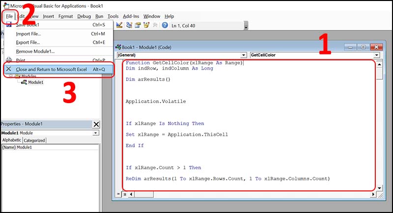
Following are the steps to set up VBA to execute the commands:

Step 1 : Open the Excel spreadsheet and press Alt + F11 to open the Visual Basic Editor (VBE).

Step 2 : Right-click on Sheet1> Select Insert > Select Module .

Complete financial functions in Excel you should know Picture 22

Step 3 : Enter the code> Select File > Select Close and Return to Microsoft Excel .

Code Function GetCellColor

 

Code Function GetCellFontColor

Code Function CountCellsByColor

Code Function SumCellsByColor

Code Function CountCellsByFontColor

Code Function SumCellsByFontColor

Code Function WbkCountCellsByColor

Code Function WbkSumCellsByColor

Complete financial functions in Excel you should know Picture 23

After completing the above steps we can use the functions to count and sum cells by color. Specifically, the properties and usage of the functions are as follows:

- GetCellColor

Usage : Returns the color code of the background color of a specified cell.

Formula : GetCellColor (Cell needs to get color code)

Example : When we need to get the background color of a red cell, we use the GetCellColor function. When entering the formula = GETCELLCOLOR (C2) (1), we will get 255 (2).

Complete financial functions in Excel you should know Picture 24

- GetCellFontColor function

Usage : Returns the color code of the font color of a specified cell.

Formula : GetCellFontColor (Cell to get color code)

Example : When you need to get the color code of a red font, you use GetCellFontColor. When you enter the formula GETCELLFONTCOLOR (C2) (1), you will get 255 (2).

Complete financial functions in Excel you should know Picture 25

- CountCellsByColor function

Usage : Counts cells with specified background color.

Formula : CountCellsByColor (Area to count, Color code to count)

Example : When we need to count the number of red cells in a selection from A1 to A15, we use the CountCellsByColor function. When you enter the formula CountCellsByColor ($ A $ 1: $ A $ 15, C2) (1) we will get 4 (2).

Complete financial functions in Excel you should know Picture 26

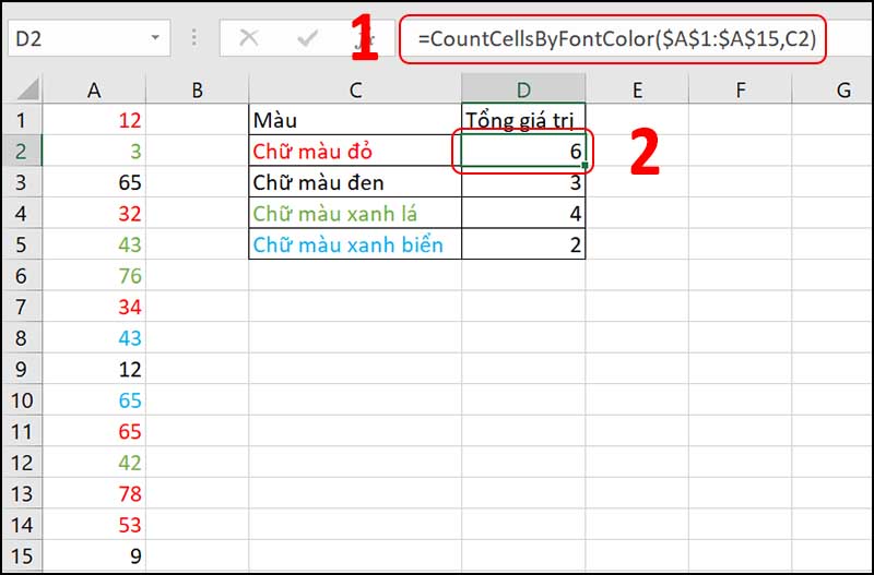
- Function CountCellsByFontColor

Usage : Count cells with the specified font color.

Formula : CountCellsByFontColor (Area to count, Color code of the font to be counted)

Example : When we need to count the number of cells with red fonts in a selection from A1 to A15, we use the CountCellsByFontColor function. When entering the formula CountCellsByFontColor ($ A $ 1: $ A $ 15, C2) (1) we will get 6 (2).

Complete financial functions in Excel you should know Picture 27

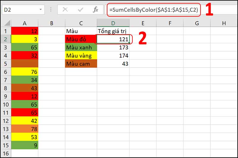
- SumCellsByColor function

Usage : Sum the cells with a certain background color.

Formula : SumCellsByColor (Area to be counted, Color code of the cell to be counted)

Example : When we need to sum values ​​of cells with the same red color in the range A1 through A15, we use the SumCellsByColor function. When you enter the formula SumCellsByColor ($ A $ 1: $ A $ 15, C2) (1), you will get 121 (2).

Complete financial functions in Excel you should know Picture 28

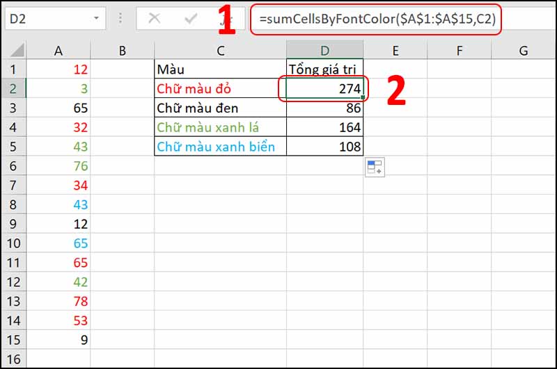
- SumCellsByFontColor function

Usage : Returns the sum of cells with a certain font color.

Formula : SumCellsByFontColor (Area to count, Color code of the font to be counted)

Example : When we need to sum values ​​of cells with the same red font in the range A1 through A15, we use the SumCellsByFontColor function. When entering the formula SumCellsByFontColor ($ A $ 1: $ A $ 15, C2) (1) we will get 274 (2).

Complete financial functions in Excel you should know Picture 29

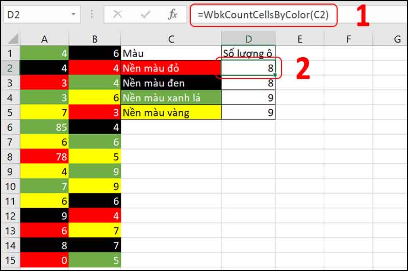
- WbkCountCellsByColor (cell) function

Usage : Counts cells with specified background color in the whole worksheet.

Formula : WbkCountCellsByColor (Cell to count)

Example : When we need to count cells with the same red background in the entire worksheet, we use the WbkCountCellsByColor function. When entering the formula WbkCountCellsByColor (C2) (1) we will get 8 (2).

Complete financial functions in Excel you should know Picture 30

- Function WbkSumCellsByColor (cell)

Usage : Sum cells with specified background color in the whole worksheet.

Formula : WbkSumCellsByColor (Color-coded Cell)

Example : When we need to count cells with the same red font in the whole worksheet, we use the WbkCountCellsByColor function. When entering the formula WbkCountCellsByColor (C2) (1), we will get 98 (2).

Complete financial functions in Excel you should know Picture 31

Hopefully the article will help you know how to use financial functions in Excel. Thank you for watching. See you in the following articles!