The 10 most useful but often forgotten functions in excel

Besides the classic Excel functions that are commonly used and used as SUM, SUMIF, IF, COUNTIF, . there are also extremely useful but less used functions such as LEFT, TRIM, MID, . How to use and meaning those functions? Let's find out in the following article

1. The TRIM function

a) Meaning

The TRIM function is a function that removes all spaces in the input text and keeps a space between words.

b) Syntax

= TRIM (text)

+ text is the paragraph, the text to remove spaces, required parameters.You can enter text or reference directly.

c) Example

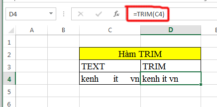
- Remove white space in the text "kenh it vn"

The 10 most useful but often forgotten functions in excel Picture 1

2. LOWER function

a) Meaning

The LOWER () function converts all characters in a text string into lowercase.

=> This function is often used when you need to reformat a sentence (usually by copying somewhere pasted into Excel) in which, lowercase letters are typed or changed wildly .

b) Syntax

= LOWER (text)

+ text: A string, or reference to a string to be formatted

c) Example

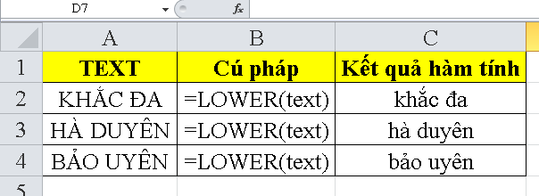
The following formula will change the words in column A to be all lowercase

= LOWER (A2) → A2: multi engraving

= LOWER (A3) → A3: ha charm

= LOWER (A4) → A4: Privacy

The 10 most useful but often forgotten functions in excel Picture 2

3. UPPER function

a) Meaning

The UPPER () function converts all characters in a text string to uppercase.

b) Syntax

= UPPER (text)

+ text: is a string, or reference to a string to be formatted.

c) Example

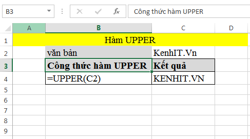
The following formula will concatenate the text string in cell C2 into text in uppercase

= UPPER (C2) → C4: KENHIT.VN

The 10 most useful but often forgotten functions in excel Picture 3

4. Function PROPER

a) Meaning

The PROPER () function converts the first character in a text of a text string to uppercase, while all the remaining characters in that string become lowercase.

b) Syntax

= PROPER (text)

+ text: A string, or reference to a string to be formatted

c) Example

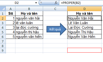
The following formula will reformat the text string from column B2-B6 from the lower case letters to the first character in a word to uppercase.

The 10 most useful but often forgotten functions in excel Picture 4

5. The SMALL function

a) Meaning

The SMALL () function is a calculation function in excel that produces the smallest k-value of a data set

b) Syntax

= SMALL (array, k)

Inside:

+ Array is an array or range of numeric data that you want to determine its kth smallest value.

+ K is the position (from the smallest value) in the array or range of data to return.

*Attention:

- The arguments of the calculation function are required values

- In case the array is empty then the SMALL function will give the #NUM! Error result..

- In case k is less than or equal to 0 or if k exceeds the number of data points, then the SMALL function will produce the #NUM! Error result .

c) Example

In part 6

6. LARGE function

a) Meaning

The LARGE () function is a calculation function in excel that produces the k-largest value of a data set

b) Syntax

= LARGE (array, k)

Inside:

+ array: An array or range of data containing the kth largest value in it.

+ k: What is the largest position (the largest adjective is No. 1) in the array you want to return.

* Attention

- If the argument in the array is a blank -> the function returns the #NUM! Error value .

- If k ≤ 0 or k is greater than the number of data points in the array -> the function returns the #NUM! Error value

- If n is the number of data points of the array, then:

+ LARGE (array, 1) -> returns the largest value in the array array.

+ LARGE (array, n) -> returns the smallest value in the array array.

c) Example

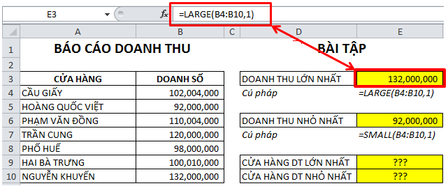
In the data table 'REVENUE REPORT' the following stores.Find stores with the largest and smallest sales

+ The largest revenue = LARGE (B4: B10,1)

+ Minimum revenue = SMALL (B4: B10,1)

The 10 most useful but often forgotten functions in excel Picture 5

7.MIN function

a) Meaning

The MIN () function is used to get the minimum value in a column.

Note: Values ​​can be numeric or string, characters, etc.

b) Syntax

= MIN (number1, number2 .)

+ number1, number2 . are input parameters that can be numbers, names, ranges of cells or reference values.Maximum 256 input parameters.

* Attention

-If the argument list contains no numbers, the Min function returns a value of 0.

-If the argument is an array or reference, only numbers in that array or reference are used.And empty cells, logical values, or text are ignored.

-The argument is text or the error value does not convert into numbers then the error function.

-The logical values ​​and numbers of text you enter directly into the argument list will be calculated.

c) Example

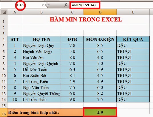
Give the following data table.Find ventricular click

= MIN (C5: C14) => is 4.9

The 10 most useful but often forgotten functions in excel Picture 6

8. The MAX function

a) Meaning

The MAX () function is used to get the maximum value in a column.

Note: Values ​​can be numeric or string, characters, etc.

b) Syntax

= MAX (number1, number2 .)

+ number1, number2 . are input parameters that can be numbers, names, ranges of cells or reference values.Maximum 256 input parameters.

* Attention

-If the argument list does not contain numbers, the Max function returns a value of 0.

-If the argument is an array or reference, only numbers in that array or reference are used.And empty cells, logical values, or text are ignored.

-The argument is text or the error value does not convert into numbers then the error function.

-The logical values ​​and numbers of text you enter directly into the argument list will be calculated.

c) Example

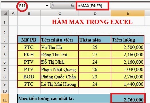
Give the following data table.Find the highest salary

= MAX (E4: E9 => is 2,760,000

The 10 most useful but often forgotten functions in excel Picture 7

9. MID function

a) Meaning

The MID function cuts out n characters in the string from the original position m

b) Syntax

= MID (text, m, n)

+ text: string to cut.

+ m: The starting position of the string to cut.

+ n: Number of characters to cut from the string.

*Attention

+ num_chars: unlike LEFT and RIGHT functions, if equal to 1, you can skip writing but with MID function, it is required to write to understand the function to get the desired number of characters.

+ When you give a topic that takes the middle character, you must use the MID function

+ The MID function can be combined with the VLOOKUP function in each case for the lesson we use.

c) Example

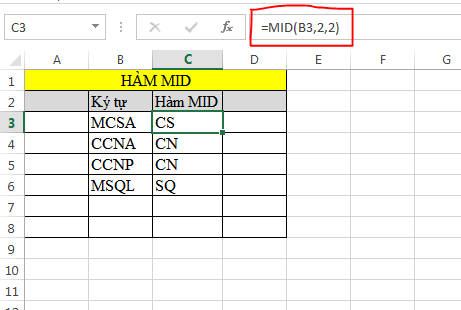
For the data table. From the character column we will start from the 2nd character and get 2 characters

The 10 most useful but often forgotten functions in excel Picture 8

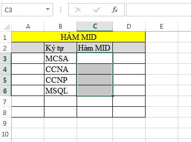
We will try to execute the MID function: = MID (B3,2,2) We will get the character CS and we just copy the formula will get the same result.

The 10 most useful but often forgotten functions in excel Picture 9

10. LEFT function

a) Meaning

LEFT () function to retrieve n characters from the left of the string (Text)

b) Syntax

= LEFT (String, [Number of characters])

+ Text: A text string containing the characters to be removed.

+ Number of characters: The number of characters to be removed from the left of the given String.

* Attention

- The number of characters retrieved must be greater than or equal to zero.

- If the number of characters retrieved is greater than the length of the text, the Left () function will return the entire text.

- If the number of characters removed is blank, it is assigned a default value of 1.

c) Example

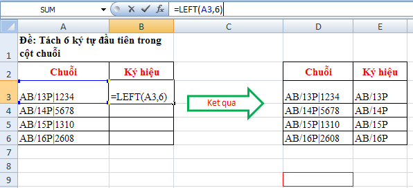
Split first 6 characters in string column

= LEFT (A3,6)

The 10 most useful but often forgotten functions in excel Picture 10