How to use the SUMIF function in Excel

Introduce

The SUMIF function is a function used to sum values ​​in a specified range. The SUMIF function can be used for summing cells based on the date, data and text that are connected to the specified area. This function supports logical operations (>, <, <>, =) and symbols (*,?) To suit each section.

Purpose

Sum the numbers in the range that meet the criteria provided.

Search for value

Total value provided.

Syntax

= SUMIF (range, criteria, [sum_range])

Parameters

Range : Range of cells you want to evaluate according to criteria. The cells in each range must be numbers or names, arrays or references containing numbers. Empty values ​​and text values ​​are ignored. The selected range may contain dates in the standard Excel format.

Criteria : Criteria for determining added values.

Sum_range : (optional) Values ​​are appended. If sum_range is removed, the cells in the scope of the evaluation will be replaced.

Attention

• When sum_range is ignored, cells in the range will be added.
• A defined area containing mathematical symbols or symbols must be enclosed in quotation marks.
• The range of numeric format that can be supplied is the number that will not have to use parentheses.
• The characters?and * can all be used in Criteria.A question mark matches any single character;an asterisk matches any character string.If you want to find a real question mark or asterisk, type the tilde (~) before the character.

How to use SUMIF in Excel

Let's explore the SUMIF calculation.

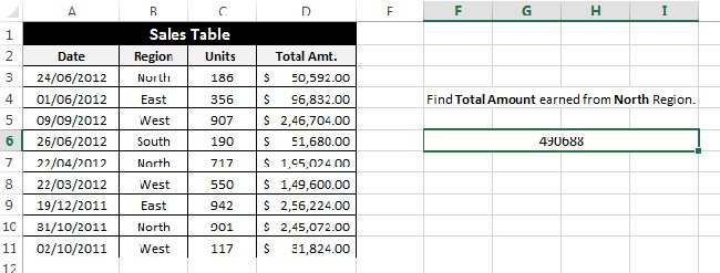
Suppose we have the following revenue table:

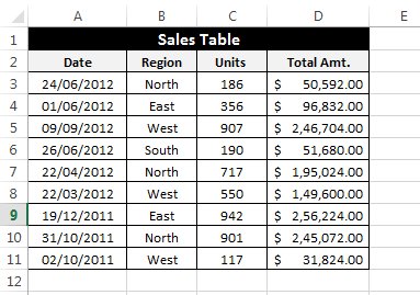
Exercise : To find the total revenue of the northern region.

Try applying the SUMIF function to solve the problem.

Range : Select the column containing "North"

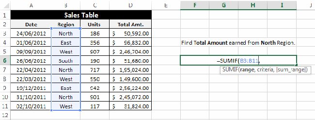
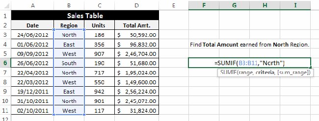
Criteria : Enter the "North" area - North. Note: Entering "North" or "= North" is fine.

Sum_range : Select the column to be added after evaluating the criteria.

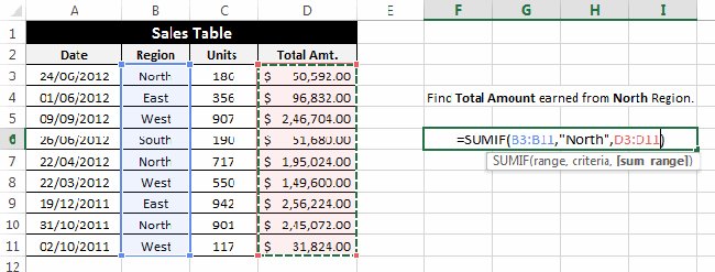
After applying this calculation, our results are 490688, the sum of D3, D7, D10.

A few examples of SUMIF

Example 1: Suppose there is a table as follows and we need to find the total quantity sold in the Eastern region.

To find the result, we need to apply the calculation: = SUMIF (B3: B11, "East", C3: C11)

And the calculation result is 129.

Example 2: In the same revenue table, write the formula to calculate the total amount before the "January 1, 2013".

In this case, we use the calculation: = SUMIF (A3: A11, "

Example 3: In this example, we have a list of items by some schools participating in regional events. The task is to find the total number of C medals achieved in events.

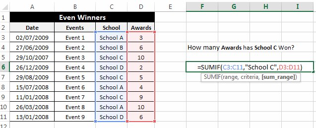
We use calculation = SUMIF (C3: C11, "School C", D3: D11)

And yes D5 + D7 + D9 has results 24.