10 good and useful Office tips

Network Administration –In this article we will summarize and introduce 10 tips that are good and useful in the field of Office.

1. Edit the word document in Print Preview mode

Print Preview allows you to check documents before printing. You can see everything, from formatting, columns, photos, headers, footers, etc. Would you be more interesting if you could change it right here, in Print Preview mode? The answer is that you absolutely can do that. Simply click the Magnifier icon in the Print Preview status bar to disable the tool. In Word 2007, uncheck Magnifier in the Preview group on the Print Preview toolbar. When done, the mouse pointer will remain in the position you edited in Normal view.

The way to do it is a little changed in Word 2010. You need to add the Print Preview Edit Mode command to the Quick Access Toolbar . The next steps are not exactly the same as those introduced above but are almost the same.

2. Find and replace how to insert a new piece of text

Search and replace tips (Find and Replace) are always popular because they bring a lot of convenience, such as inserting a new piece of text. For example, to insert a new changed title after the places where your name appears in the document, you can find the name and insert the changed title, but there is a way. simpler: Use the ^ command & in the Replace With value.

The ^ & command will make the Find and Replace tool insert the text in the Find What entry after your name. In the recent simple name example, you can use the following settings:

Find What: John Doe

Replace With: ^ &, MCSE

You can use this technique to insert a piece of text before and after a pre-existing string.

3. Insert a comparison chart into the worksheet

Excel is a very smart application for charting, but sometimes you don't want to use all of that, just want to compare values ​​visually. For example, the worksheet shown in Figure A lists the number of products sold by each person. Since the list is still short, you can take a quick look and discover that the person named Bill sold the most products and Kate sold the least. If all you need is to quickly find out what is the highest value and what is the lowest value in a long list, this type of display cannot help you compare values. This is the time you use bar charts to create visual comparisons. They look complicated but are the result of Excel's REPT () function.
In cell C2, we have entered the function below:

= REPT ('|', B2)

We then copied this function to C3: C9. The results will allow you to visually compare each value to each other. This is a very good and easy-to-follow tip, the results are very clear.

10 good and useful Office tips Picture 1
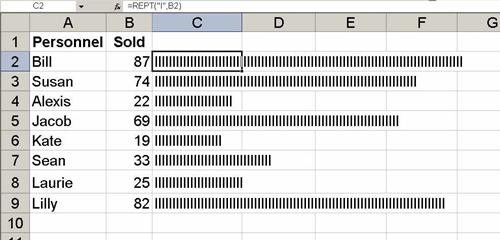
Figure A: Use the REPT () function to create a visual comparison chart

In Excel 2010, you can create a similar effect by using sparkline s . The REPT () function will be faster and easier, but sparklines are more flexible and flexible.

4. Remove the background image of the company logo

Adding a company logo to a PowerPoint presentation seems like a very simple task. However, these graphic files often show up with a background image, and unless the slide background image matches the logo's background image, this overlap is unacceptable. If your logo is a bitmap file, the solution here is simple but some of you may not know yet:

1. In the Normal view, right-click on the logo image and select Show Picture Toolbar to display the Picture toolbar.
2. Click the Set Transparent Color tool (the button near the end). The cursor will change the transparency of the transparent tool.
3. Click on the background image. If you're lucky, the background image will magically disappear!

If you use PowerPoint 2007 or 2010, follow these steps:

1. Click the Format tab.
2. In the Adjust group, select Set Transparent Color from the Recolor drop-down list.
3. Click the background of the image.

You can use this feature to remove other background images. Just click on a certain area and it will disappear. If you don't like how to change it, press [Ctrl] + Z. The worst thing, you may have to delete and reinstall the file to start over. This transparent setting works best with bitmaps.

5. Add indicator tape to a PowerPoint slide

Using the Print Crawl feature in PowerPoint, you can turn a normal text box into a ticker tape readout. There is a trick in this technique, but it's easy to do that - you have to locate the text box in an unusual way. The steps below are used in PowerPoint 2003:

1. Add a text box to the slide and type the message you want to roll.
2. Here's how: Drag the text box down to the bottom left of the slide, as shown in Figure B. You should use the right side to maintain the slide. By moving most text boxes from the slide, you will allow your text to run from the left corner.
3. Right-click on the text box and select Custom Animation .
4. Select Entrance from the Add Effect list and select More Effects .
5. Select Crawl Print from the list of basic effects and click OK .
6. Change the Start setting to After Previous .
7. Change Direction setting to From Right .
8. Change Speed setting to Very Slow .
9. From the list of drop-down effects, select Timing .
10. From Repeat list, select Until End Of Slide .
11. Click OK .

10 good and useful Office tips Picture 2

Figure B: Drag the text box to the side of the sdile

Press F5 and see the message you entered in the text box that runs into the screen from the right, run through the bottom edge and to the left side of the slide.

You can adjust the time slightly. The word run can be changed quickly or slowly to make the reader not lose interest.

6. Add the total values ​​in the filtered Excel list

Using filters, you can filter out the data you need to see. However, adding up the filtered records is another matter. Figure C shows a filtered list. You can see the filtered item on the left. The problem is that the SUM () function does not return the expected result for you because it evaluates all values ​​in D14: D64, not just the existing values. There is no way to allow the SUM () function to know that you only want to value filtered values ​​in the reference range.

10 good and useful Office tips Picture 3
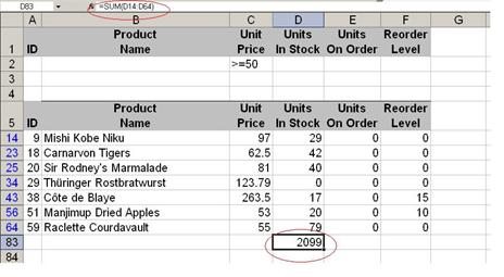
Figure E: The SUM () function does not work as expected with the filter list

The solution here is much simpler than what you think. You just need to click AutoSum and Excel will automatically enter a SUBTOTAL () function instead of the SUM () function. This function will look at the entire list, D6: D82, but it specifies the price of the filtered values, as shown in Figure D.

10 good and useful Office tips Picture 4
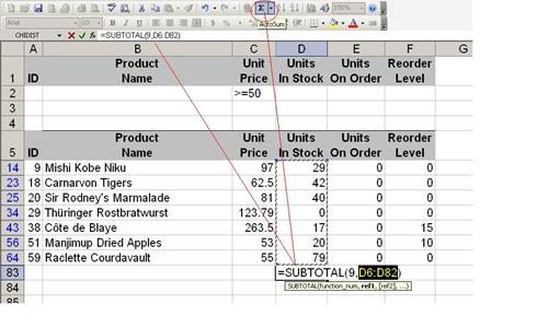
Figure D: SUBTOTAL () function evaluates the existing values ​​in the filter list

7. Fill in empty cells in Excel

In a spreadsheet, a lot of gaps appear to create a confusing feeling for the reader. If you don't like a cool page with such empty cells, you can use the steps below to fill in something.

10 good and useful Office tips Picture 5
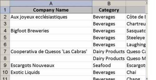
Figure E: The spaces in the CompanyName field confuse readers.

1. First, select a range of white characters that you need to replace with other characters. Do not select column header cells - select only the range containing the actual data. Using the worksheet above, the actual data range is A2: A11 .
2. Select Go To from the Edit menu or press [Ctrl] + G and then click the Special button. In Excel 2007, select Go To Special from the Find And Select list in the Editing group on the Home tab.
3. Select Blanks and click OK . Excel will select all white cells in A2: A11.
4. In the first selected white cell (A3), enter an equal sign and point to the upper cell. Cell has been selected, you do not have to click A3.
5. Press [ Ctrl] + [Enter] , Excel will copy the formula equivalent to all white cells in the selected range.

At this point, the range will contain text values ​​(original values) and formulas that repeat the values ​​in that word. To replace the formulas with their results, select the range (A2: A11) and select Copy from the Edit menu. In Excel 2007, click Copy in the Clipboard tab.

Select Paste Special from the Edit menu. Then select Values and click OK . In Excel 2007, select Paste Values from the Paste list in the Clipboard group on the master tab. Now you have replaced the formulas with text values, as shown in Figure F.

10 good and useful Office tips Picture 6
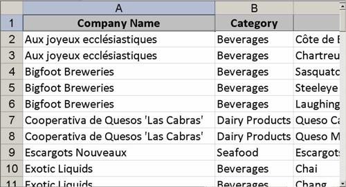
Figure F: Empty cells are now the company name

8. Insert watermark into word document

A watermark is an image or text that appears behind the contents of a document. It usually has some gray or neutral color to not affect the purpose of the document. Typically, a watermark identifies a company or document status. For example, a watermark may say confidential (urgent), urgent (urgent) or display a graphic icon. Inserting watermark into word document is a simple process and in this article we will show you how to do this:

1. Click the Page Layout tab
2. Click Watermark in the Page Background group
3. Select a watermark from the library. Or…
4. Select Custom Watermark . The Printed Watermark dialog box will appear with three options. You can remove a custom watermark or insert a certain image or text as a new watermark.

5. Click OK when you're done with your selection.

If you're using Word 2003, you can insert a watermark in the following way:

1. From the Format menu, select Background .
2. Click Print Watermark.
   To insert an image as a watermark, click Picture Watermark. Then click Select Picture , navigate to find the image file, and then click Insert .
   To insert a text, click Text Watermark and select or enter the text you want.
3. Set up additional options.
4. Click OK

The watermark will display as a background of each page and your results will be as shown in Figure G below.

10 good and useful Office tips Picture 7
Figure G: Watermark is an effective way of sharing information about the status or purpose of a document

9. Get the sum using Excel's status bar

Have you ever encountered a situation when you're in a meeting and someone who is very important to ask about the total or number of shortages that you don't have in your spreadsheet? This time will be very awkward for you! Everyone looks at you while you enter an appropriate function. Although this period will not be long, it makes you feel that you are inferior, despite the fact that you are not such a person.

If you are lucky, you can simply select the first white box near the column or row and click AutoSum. This is not so bad, but what if someone wants you to give a valuation to a subset? Maybe they want to know sales in the first and second quarter in both the South and the North. Certainly this job will make you lose more action - and when under psychological pressure, you are very likely to make mistakes.

One way you can quickly evaluate certain values ​​is to use the Status bar. You can add or take an average of a range of values ​​without entering anything. You only need to specify the minimum and maximum values ​​in the range. You can even count the number of entries in a range, all without entering a function or a formula.

Select the values ​​in question and observe the right side of the Status bar. For example, to see sales for both the South and the North in the first and second quarter in the worksheet shown in Figure H, select B2: C3. When performing this operation, the Status bar will display:

Sum = $ 1,415.10

on the left of the NUM indicator. Note that the Status bar will indicate the total value of the selected range and many other options by right-clicking on the Status bar and selecting the appropriate option from a list of activities. Using this utility, you will get answers in a few clicks. No one has to wait for you and now you will become more confident and calmer!

10 good and useful Office tips Picture 8
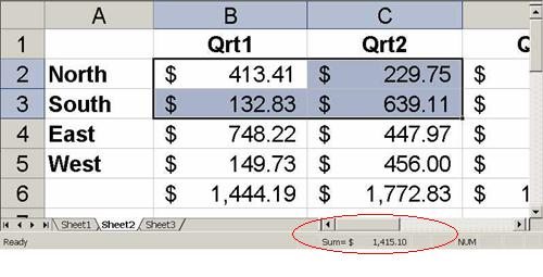
Figure H: Use the calculation tool in Status bar

10. Create an email shortcut to facilitate mail delivery

Most of your email notifications usually come from someone - sometimes you can send a few times a day to someone. Normally, entering the same address is not effective, even we have Outlook's AutoComple feature. If you send a lot of emails to the same person, create an email shortcut on your desktop. When you want to send a message, just double-click the shortcut to open a previously addressed message but there is no content. Then what you do is write the content for it and press the Send button.

To create a desktop shortcut for sending messages to the same person, you can do it the following way:

1. Right-click the desktop and select New , then select Shortcut .
2. In the Create Shortcut dialog box, type mailto: emailaddress . Do not enter any empty characters between the mailto: and email addresses.
3. Click Next and enter a descriptive name for the shortcut.
4. Click Finish .

To use a new shortcut, double-click it. Outlook (or your default email client) will open a mail window and fill in the To field using the address you provided when creating the shortcut. Write the content and press Send! This is an interesting solution for making sure email arrives at the right recipient if you have two or more names with contacts.