Steps to create relationships between multiple tables using Data Model in Excel

Thanks to the Excel Data Model, you can save valuable time through automated data reports. Learn how easily you can assign a relationship between two tables using the Data Model and illustrate that relationship in the following article.

Basic Requirements

You will need Power Pivot and Power Query (Get & Transform) to complete some tasks while creating the Excel Data Model. Here's how you can get these features in your Excel workbook:

How to get Power Pivot

1. Excel 2010: You need to download the Power Pivot add-in from Microsoft, then install it for the Excel desktop program.

2. Excel 2013: The Office Professional Plus version of Excel 2013 includes Power Pivot. However, you need to activate it before using it for the first time. Here's how to do it:

1. Step 1: Click File on the ribbon of the Excel workbook.
2. Step 2: Then click Options to open Excel Options.
3. Step 3: Now, click on Add-ins.
4. Step 4: Select COM Add-ins by clicking the drop-down menu of the Manage box .
5. Step 5: Click Go and then select the check box for Microsoft Power Pivot for Excel .

Steps to create relationships between multiple tables using Data Model in Excel Picture 1

Step 3. Excel 2016 and later: You will find the Power Pivot menu on the ribbon.

How to get Power Query (Get & Transform)

Step 1. Excel 2010: You can download the Power Query add-in from Microsoft. Once installed, Power Query will show up on the ribbon.

Step 2. Excel 2013: You need to enable Power Query by following the same steps you just did to get Power Pivot working in Excel 2013.

Step 3. Excel 2016 and later: You can find Power Query (Get & Transform) by going to the Data tab on the Excel ribbon.

Create Data Model by importing data into Excel Workbook

For this tutorial, you can get preformatted sample data from Microsoft:

1. Download Sample Student Data (data only) | Sample student data (complete model)

You can import a database with many related tables from many sources such as Excel workbooks, Microsoft Access, web pages, SQL Server, etc. Then you need to format the data set so that Excel can use it. Here are the steps you can try:

Step 1. In Excel 2016 and later, click the Data tab and select New Query.

Step 2. You will find several ways to import data from external or internal sources. Choose a way that suits you.

Steps to create relationships between multiple tables using Data Model in Excel Picture 2

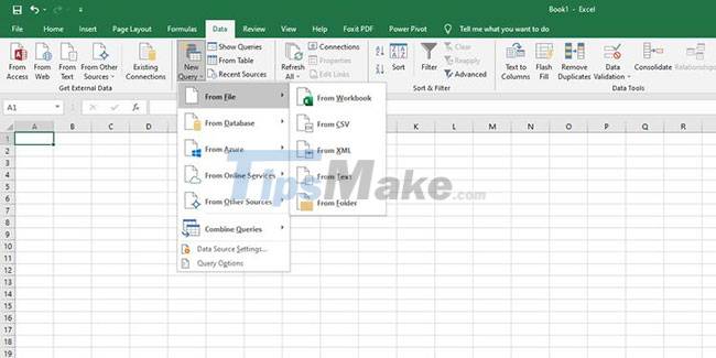
Step 3. If using the Excel 2013 version, click Power Query on the ribbon and then select Get External Data to select the imported data.

Step 4. You will see a Navigator box where you need to select which tables you need to import. Click the Select multiple items to pick several tables for import checkbox .

Steps to create relationships between multiple tables using Data Model in Excel Picture 3

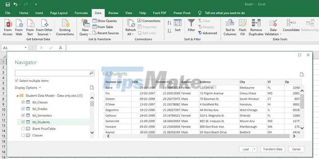
Step 5. Click Load to complete the import.

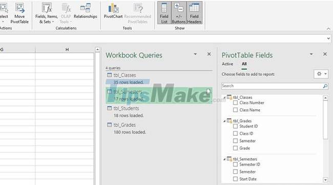
Step 6. Excel will create the Data Model for you using these tables. You can see the table column headers in the PivotTable Fields list .

Steps to create relationships between multiple tables using Data Model in Excel Picture 4

You can also use Power Pivot functions like calculated columns, KPIs, hierarchies, calculated fields, and filtered data sets from the Excel Data Model. For this purpose, you will need to create a Data Model from a table. You can try the following steps:

Step 1. Format the data in a tabular model by selecting all cells containing the data and then clicking Ctrl + T .

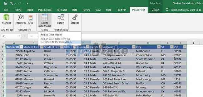
Step 2. Now select the entire table and then click the Power Pivot tab on the ribbon.

Step 3. From the Tables section , click Add to Data Model .

Steps to create relationships between multiple tables using Data Model in Excel Picture 5

Excel creates a tabular relationship between related data from the Data Model. For this, primary and foreign key relationships are required in the imported tables.

Excel uses the relationship information from the imported table as a foundation to create connections between the tables in the Data Model.

Building relationships between tables in Data Model

Now that you have the Data Model in your Excel workbook, you'll need to define the relationships between the tables to generate meaningful reports. You need to specify a unique field identifier or primary key for each table, like Semester ID, Class Number, Student ID, etc.

Power Pivot's Diagram View feature lets you drag and drop those fields to build relationships. Follow these steps to create a table link in Excel Data Model:

Step 1. On the ribbon of the Excel workbook, click the Power Pivot menu .

Step 2. Now, click Manage in the Data Model section. You will see the Power Pivot editor as shown below:

Steps to create relationships between multiple tables using Data Model in Excel Picture 6

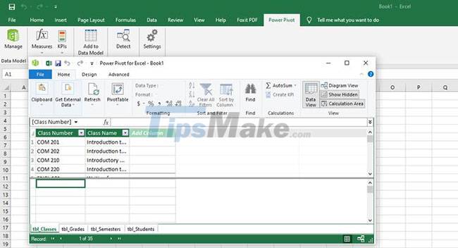
Step 3. Click the Diagram View button located in the View section of the Power Pivot Home tab . You will see the column headings in the table grouped by the table name.

Steps to create relationships between multiple tables using Data Model in Excel Picture 7

Step 4. You can now drag and drop the unique field identifier from one table to another. The following is the relationship diagram between the 4 tables of Excel Data Model:

Steps to create relationships between multiple tables using Data Model in Excel Picture 8

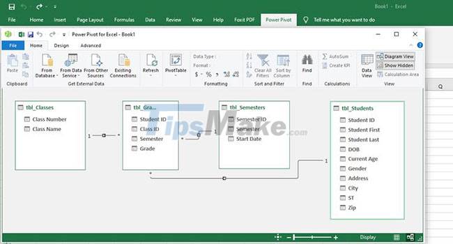
The following describes the relationship between the tables:

1. Students Table | Student ID to Grades table | Student ID
2. Table Semesters | Semester ID to Grades table | Semester
3. Table Classes | Class Number to Grades table | Class ID

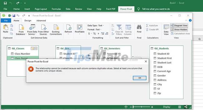
Step 5. You can create a relationship by selecting a unique pair of column values. If there are any duplicates, you will see the following error:

Steps to create relationships between multiple tables using Data Model in Excel Picture 9

Step 6. You should see an asterisk (*) on one side and a number (1) on the other in the Diagram View of the relationships. It defines that a one-to-many relationship exists between the tables.

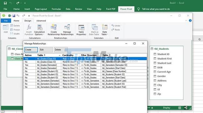
Step 7. On the Power Pivot editor, click the Design tab and then select Manage Relationships to see which fields make the connection.

Steps to create relationships between multiple tables using Data Model in Excel Picture 10

Create PivotTable with Excel Data Model

You can now create a PivotTable or PivotChart to visualize your data from the Excel Data Model. An Excel workbook can contain only one Data Model, but you can keep updating the tables.

Because the data changes over time, you can continue to use the same model and save time when working with the same data set. You'll find yourself saving more time when working on data with thousands of rows and columns. To create a report based on a PivotTable, follow these steps:

Step 1. On the Power Pivot editor, click the Home tab .

Step 2. On the ribbon, click PivotTable.

Step 3. Select New Worksheet or Existing Worksheet.

Steps to create relationships between multiple tables using Data Model in Excel Picture 11

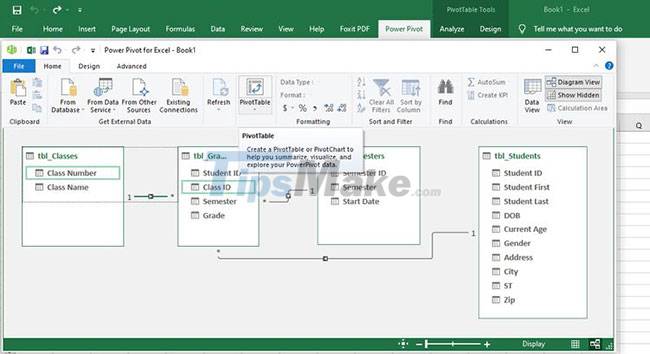
Step 4. Select OK. Excel adds a PivotTable that displays the Field List panel on the right.

Steps to create relationships between multiple tables using Data Model in Excel Picture 12

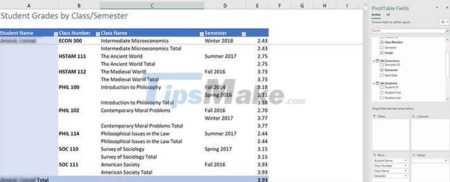
The following is an overview of the table created using the Excel Data Model for sample student data used in this tutorial. You can also create professional-looking pivot tables or charts from big data using the Excel Data Model tool.

Hope you are succesful.

Kareem Winters

Update 03 June 2021