How to Use the VLOOKUP Function in Excel

This guide explains how to use VLOOKUP Function in Excel, including its syntax, required arguments, practical examples, and common errors.

1. Syntax and usage of VLOOKUP function

- VLOOKUP function is a search for conditional values, the search is performed on columns.

- VLOOKUP function syntax:

VLOOKUP (lookup_value, table_array, col_index_num, [range_lookup])

Inside:

+ lookup_value: The value you want to search, is a required parameter.

+ table_array: The data area you want to search for values, is a required parameter.

+ col_index_num: Column containing the value to search, is a required parameter.

+ range_lookup: Search type, range_lookup = 1 is equivalent to True value -> relative search, range_lookup = 0 absolute search is equivalent to false value.

2. Simple example using VLOOKUP function

2.1 Example 1

- The following data sheet is available, based on the allowance allowance sheet filled out for employees (using Vlookup function):

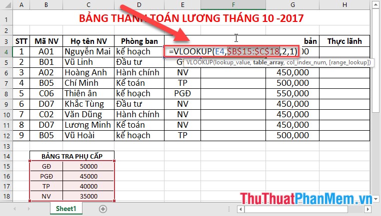
- In the cell to calculate the formula entry allowance: = VLOOKUP (E4, $ B $ 15: $ C $ 18,2,1) (note the absolute value for the data range containing the search value):

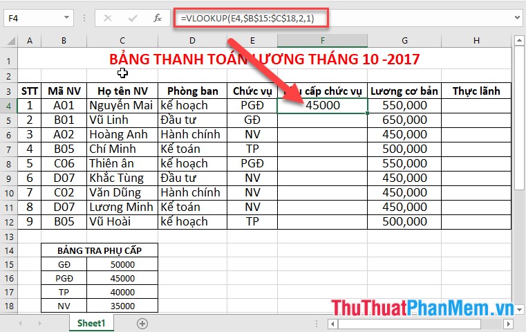
- Press Enter to get the results:

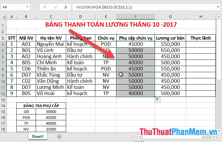
- Similarly copying the formula for the remaining values results:

2.2 Example 2

- Enter employee qualifications based on the employee code, if the employee is on the qualification table

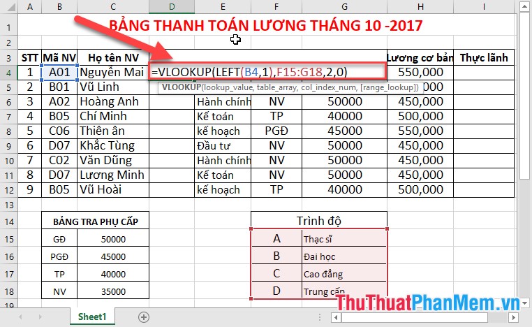
- Here to get the employee qualifications through the first character in the staff code. So, you need to use the Left () function to get the first character in the code and look for that character in the level table.

- In the cell to calculate, enter the formula: = VLOOKUP (LEFT (B4,1), $ F $ 15: $ G $ 18,2,0)

- Press Enter to get the results:

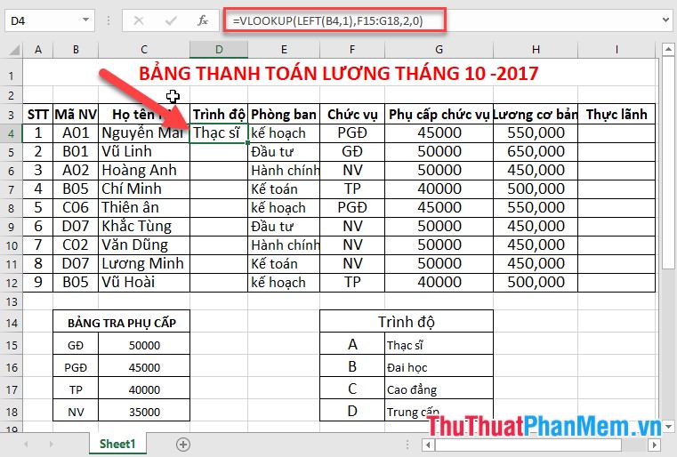
- Copying the formula for the remaining values displays the error message:

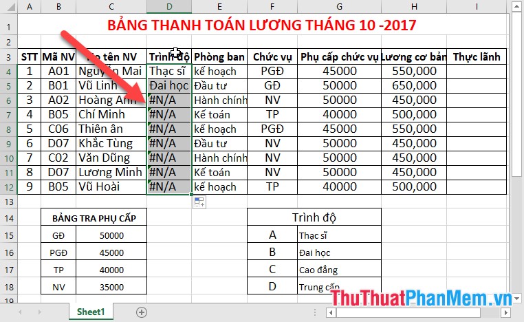
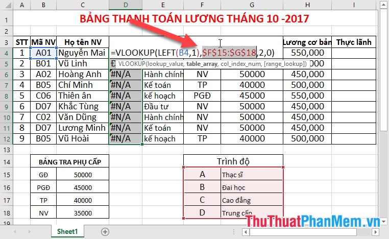
- Because of not placing an absolute address for the data area containing the search value, VLOOKUP function reports an error, executes the address highlight, and press F4 key to change the address to the absolute address:

- Finally copying the formula to the remaining values results:

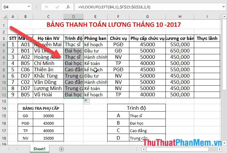
2.3 Example 3

Enter the department information and employee ranks based on the department table and category below:

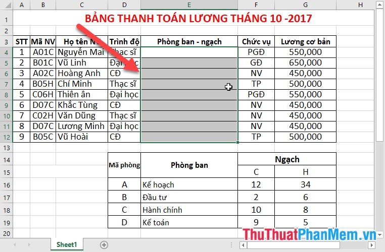
- Here to get the staff's department based on the first character in the kernel code. To get a rank based on the last character in the employee code. But here the department values are arranged in columns so VLOOKUP should be used while rows value should be used in HLOOKUP . Departments and ranks should put together 1 column and combine 2 values into 1.

In the field you need to enter the formula: = VLOOKUP (LEFT (B4,1), $ D $ 16: $ E $ 19,2,1) & "-" & HLOOKUP (RIGHT (B4,1), $ F $ 15: $ G $ 19,2,1)

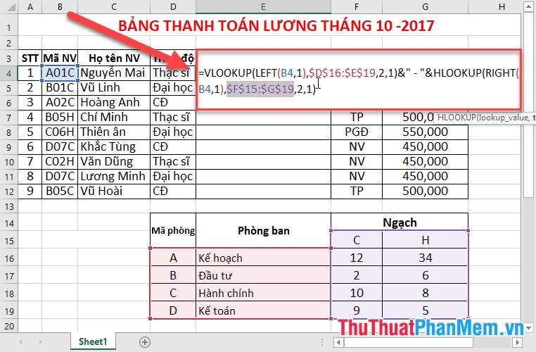
- Press Enter to get the results (remember to pass the absolute address for the search value container):

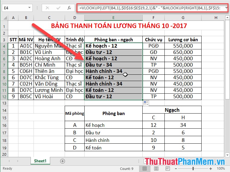
- Similarly copying the formula for the remaining values results:

The above is a detailed guide on how to use the VLOOKUP function and some specific examples that hope to help you. Good luck!