The RIGHT function in Excel: syntax and illustrative examples.

Similar to the LEFT function, RIGHT is a popular function in MS Excel used to retrieve custom data based on certain conditions. Simply put, the RIGHT function in Excel is designed to return a specified number of characters from the far right of a string. This article will provide you with complete information about the concept, formula, and usage of the RIGHT function, both independently and in combination with other functions.

What is the RIGHT function in Excel? How to use the RIGHT function and illustrative examples.
 

Article Contents:
1. Benefits of using the RIGHT function
2. Syntax of the RIGHT function in Excel
3. Specific examples using the RIGHT function in Excel
4. How to use the RIGHT function in Excel
     4.1 Extracting a string of characters following a specific character
     4.2 Extracting a string after the last separator
     4.3 How to remove the first N characters in a string
     4.4 The Excel RIGHT function can return a zero value
     4.5 Why the RIGHT function doesn't work with date values
​​5. Some errors with the Excel RIGHT function: Function not working and solutions

 

1.  What is the Right function in Excel?

RIGHT is a text string function in Excel that extracts characters starting from the far right and working towards the left. The extracted result depends on the number of characters specified in the formula.

The RIGHT function can be used alone and combined with other functions such as VALUE, SUM, COUNT, DATE, DAY, etc., to extract data that meets various conditions.

* Benefits of using the RIGHT function

+ Helps extract the desired characters from a long string, applicable to various data strings.

The RIGHT function has a very simple and easy-to-understand syntax, and can be applied to all versions of Microsoft Excel and Google Sheets.
 

2. Syntax of the RIGHT function in EXCEL

Syntax : RIGHT(text, n)

- In which : + Text : ( Required parameter) a string of characters.

                  + n : The number of characters to extract from the string.

- Function : Extracts n characters from a text string starting from the right.

A few notes: 

- The parameter n must always be greater than or equal to 0.
- If the parameter n is not specified, Excel will default its value to 1.
- If the parameter n is greater than the length of the string, the result will be the entire string.
- The RIGHT function always returns text characters. The returned characters may be numbers, and you might mistakenly think they are numbers. This is completely incorrect; although the returned values ​​look like numbers, they are still text. Depending on the specific case when combined with other functions, you will need to reformat these results to make them suitable for calculations and lookups.

3. Specific examples of using the RIGHT function in EXCEL

As a worksheet function, RIGHT can be entered as part of a formula in a worksheet cell. To better understand how to use the function, let's consider the following example:

Example 1 : String splitting without the parameter n :

Apply the RIGHT function to extract characters from the 'HS Code' column in the case where the parameter 'n' is not provided.
- In cell E5 , type the following formula: E6 = RIGHT(D6) and press Enter.
- Cell D6 contains the data you want to extract the string from.
- The result will be displayed in cell E6.

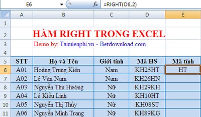
Example 2 : Extract 2 characters from the string in the ' HS Code ' column starting from the right.

We apply the RIGHT function to extract 2 characters from the ' HS Code ' column.
- In cell E6  , type the following formula: E6 = RIGHT(D6, 2) and press Enter.
- Cell D6 is the cell containing the data you want to extract the string from.
- The result will be displayed in cell E6.

 

4. How to use the RIGHT function in EXCEL

In practice, the RIGHT function is rarely used alone. More often, it's used in combination with other Excel functions in complex formulas.

4.1. Extracting the String Following a Specific Character

If you want to extract the character string following a specific character, use the SEARCH or FIND function to determine the position of that character. Subtracting the selected character's position from the returned string, use the LEN function to pull the desired number of characters from the right side of the original string.

General formula:

RIGHT(string, LEN(string) - SEARCH(character, string))

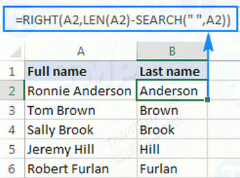
For example, cell A2 contains the first and last names separated by a space. Your goal is to move the name to another column. Apply the formula above, then enter A2 in the blank space of the string, and enter the character in the blank space '', as in the formula below.

=RIGHT(A2,LEN(A2)-SEARCH(" ",A2))

The formula above returns the following result:

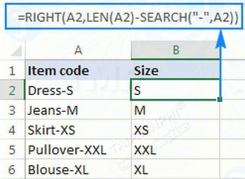
Similarly, you can extract the string following any other character, such as a comma, colon, or hyphen, etc. For example, to extract the string following the hyphen (-), you apply the formula:

=RIGHT(A2,LEN(A2)-SEARCH("-",A2))

The formula above returns the following result:

4.2. Extracting the String After the Last Delimiter

When dealing with complex strings where a delimiter appears multiple times, you often need to extract the text string after the last delimiter. To make things easier to understand, please refer to the example below:

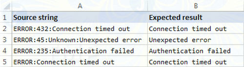
In the screenshot above, column A contains a list of error names. Your goal is to drag the error description after the colon to another column. However, it's important to note that the number of colons in the original string is different. For example, cell A3 has three colons, while column A5 has only one.

The key here is to locate the last separator (i.e., the colon in this example) in the original string. To do this, you'll need to use a combination of concatenating functions:

1. Get the number of separator characters in the original string.

First, calculate the total length of the string using the LEN function: 

LEN (A2)

The next step is to calculate the length of the string without the delimiter using the SUBSTITUTE function, replacing the colon:

LEN(SUBSTITUTE(A2,":",""))

Finally, subtract the original string length without delimiters from the total string length:

LEN(A2)-LEN(SUBSTITUTE(A2,":",""))

Make sure all the above formulas work. You can enter these formulas into separate cells, and the result will be 2, which is the number of colons in cell A2.

2. Replace the last delimiter with a unique character. To extract the text after the last delimiter in a string, you will need to mark the last delimiter with a specific character. To do this, you replace the last delimiter (i.e., the colon) with a new character that does not appear in the original string, such as (#).

If you're familiar with Excel's SUBSTITUTE function syntax, this function has a fourth optional argument (instance_num) that allows you to replace a specified character in a text string. And since the number of separator characters in the string has already been calculated, simply add the above function as the fourth argument in another SUBSTITUTE function:

=SUBSTITUTE(A2,":","#",LEN(A2)-LEN(SUBSTITUTE(A2,":","")))

If you enter the above formula into a different cell, the result returned will be the string: ERROR:432#Connection timed out.

3. Find the position of the last delimiter in the string. Depending on the character you use to replace the last delimiter, use the SEARCH or FIND function (case-insensitive) to determine its position in the string. In this example, the delimiter (i.e., the colon) is replaced with a #; the formula used to find the position of the # is below: 

=SEARCH("#", SUBSTITUTE(A2,":","#",LEN(A2)-LEN(SUBSTITUTE(A2,":",""))))

In this example, the result returned is 10, which is the position of the # symbol in the string that has been replaced.

4. Return the string to the right of the last delimiter. 

Once you know the position of the last delimiter in a string, all you need to do now is subtract that delimiter position from the total string length, and the RIGHT function will return the string to the right of the last delimiter in the original string:

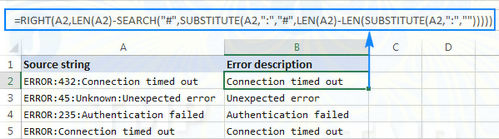
=RIGHT(A2,LEN(A2)-SEARCH("$",SUBSTITUTE(A2,":","$",LEN(A2)-LEN(SUBSTITUTE(A2,":","")))))

As you can see in the screenshot below, the recipe works quite perfectly:

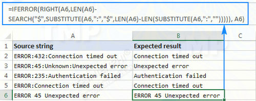
If you're working with a large dataset with many cells containing different separators, you can nest the above formula within the IFERROR function to prevent potential errors:

=IFERROR(RIGHT(A2,LEN(A2)-SEARCH("$",SUBSTITUTE(A2,":","$",LEN(A2)-LEN(SUBSTITUTE(A2,":",""))))), A2)

If a particular string does not contain the specified delimiter, the original string will be returned, as in line 6 of the screenshot below:

4.3. How to Remove the First N Characters in a String

In addition to extracting a substring from the original string, the Excel RIGHT function is also used to remove symbols from the original string.

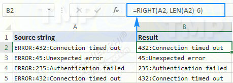
Suppose in the dataset used in the previous example, you want to remove the word "ERROR" that appears at the beginning of each string and leave only the error code number and description. To do this, simply subtract the number of characters to be removed from the total length of the original string and use that number as the num_chars argument in the Excel function RIGHT:

RIGHT(string, LEN(string)-number_of_chars_to_remove)

In this example, the first 6 characters (including 5 letters and 1 colon) are removed from the text string in cell A2 using the formula below:

=RIGHT(A2, LEN(A2)-6)

4.4. The Excel RIGHT function can return a value of zero.

As mentioned above, the Excel RIGHT function always returns a text string even if the initial value is a number. 

However, if you're working with numbers and want the result to also be a number, the simplest solution is to nest the RIGHT function within the VALUE function, which is specifically designed to convert text strings to numbers.

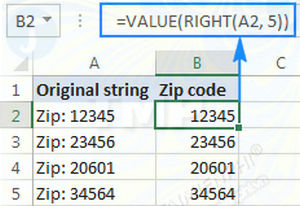
For example, to extract the last 5 characters (postal code) from the string in cell A2 and convert the extracted characters into numbers, you would use this formula:

=VALUE(RIGHT(A2, 5))

The screenshot below shows the results, revealing right-aligned numbers in column B, as opposed to left-aligned text in column A:

4.5. Why Doesn't the RIGHT Function Work with Date Values?

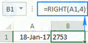
Because the Excel RIGHT function is designed to work with text strings, while dates are represented by numbers in the Excel system, the RIGHT function cannot extract individual parts like days, months, or years. If you try to use the RIGHT function to do this, all you will get are the last digits of the original string representing the date.

Let's say cell A1 contains the date January 18, 2017. If you try to use the formula RIGHT(A1,4) to extract the year, the result will be 2753, which are the last four digits of the number 42753 representing January 18, 2017 in Excel.

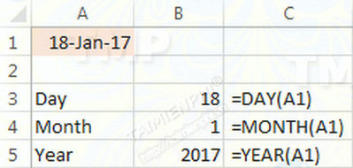
So how do you get a specific part of a day? Simply use one of the Excel functions below:
The DAY function extracts a day: =DAY(A1)
The MONTH function extracts the month: =MONTH(A1)
The YEAR function extracts the year: =YEAR(A1)

The screenshot below shows the results:

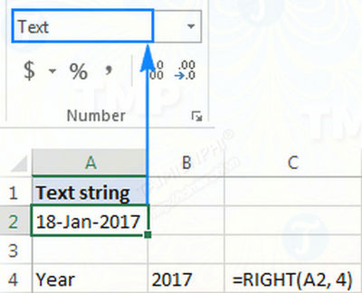
If your date is represented by a text string, which often happens when exporting data from an external source, you can use the RIGHT function to extract the last few characters in the string that represent a specific part of the date, such as day, month, year:

 

5. Some Excel RIGHT Function Errors: Functions Not Working and Solutions to Fix Them

If an Excel RIGHT function isn't working in your spreadsheet, it could be due to:
1. The original data contains one or more spaces. To remove spaces and blanks in cells, use the Excel TRIM function or the Cell Cleaner add-in.
2. The num_chars argument is less than 0. Of course, you wouldn't use negative numbers in your formula, but if the num_chars argument is calculated by another Excel function or nested Excel functions, the RIGHT function will return a #VALUE! error.
Try checking the nested functions to find and fix the error.
3. The initial value is a date. As mentioned above, the RIGHT function cannot work with dates, so if the initial values ​​are dates, the RIGHT function will return an error.

Above, we have introduced you to the Right function in Excel, which is used to extract characters from the right side of a string. Through the illustrative example, you will better understand the syntax and usage of the Right function.

Additionally, if you want to extract characters in the middle of a string, you can use the Mid function in Excel. In a long string, extracting characters in the middle is quite difficult, especially if it's a list with thousands of columns. Using the Mid function in this case will be the most efficient method.

The CONCATENATE function helps to concatenate strings in calculation columns, regardless of how much data you have in the column to be concatenated. With the CONCATENATE function , everything will be solved easily.

Do you often use the Right function in your work? If so, please share some experiences and tips on using the Right function with us by commenting below.

In addition, if you're looking to learn how to split strings in Excel, please refer to the article here.