How to Use Claude to Write and Check Excel Formulas

Claude can turn a description of a spreadsheet task into a candidate Excel formula and explain how it works. The useful part is the back-and-forth: you can clarify the layout, ask about edge cases and request a simpler alternative. You still need to test the formula in Excel before using it on important data.

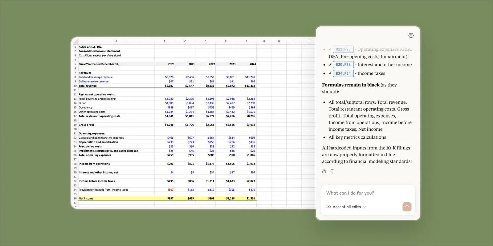
How to use Claude AI to write Excel formulas instantly. Picture 1

Describe the workbook, rule and expected result

Include your Excel version, sheet names, relevant columns, first data row and the cell where the formula will go. State how blanks, duplicates and missing matches should be handled. If your installation uses semicolons instead of commas between arguments, say so.

I use Excel 2021 with comma separators. Data starts on row 2. Column A contains salesperson names, B contains regions, and C contains revenue. In D2, calculate a bonus of 10% when revenue is strictly above 50,000, otherwise 5%. Leave D2 blank when C2 is blank. Explain the formula and give three test cases.

Paste a few invented or anonymized example rows rather than confidential customer or employee records. If you are new to cell references, review Excel formula and function basics first.

Example 1: calculate a conditional bonus

For numeric revenue in C2, this formula implements the stated rule and leaves the result empty when C2 is empty:

=IF(C2="","",IF(C2>50000,C2*10%,C2*5%))

Revenue in C2	Expected bonus	Reason
40,000	2,000	5% rate
50,000	2,500	The higher rate requires strictly more than 50,000
60,000	6,000	10% rate
Blank	Blank	The outer IF handles missing revenue

The formula assumes revenue is stored as a number. Decide separately whether negative values are valid. If the policy says “50,000 or more,” change > to >=. That one character changes the boundary result.

Example 2: look up a value using two criteria

Suppose A2:A100 contains categories, B2:B100 contains regions, and C2:C100 contains the values to return. In an Excel version supporting XLOOKUP, use:

=XLOOKUP(1,(A2:A100="Electronics")*(B2:B100="North"),C2:C100,"Not found",0)

Each comparison produces TRUE or FALSE values; multiplying the arrays identifies rows where both conditions hold. XLOOKUP returns the value for the first matching row. If you need the total for every matching row, ask for SUMIFS instead. If you need every matching record, a first-match lookup is the wrong result type.

Microsoft notes that XLOOKUP is unavailable in Excel 2016 and Excel 2019. An INDEX/MATCH alternative is:

=INDEX(C2:C100,MATCH(1,(A2:A100="Electronics")*(B2:B100="North"),0))

In older Excel versions, this array formula may require Ctrl+Shift+Enter; modern dynamic-array versions accept Enter. Use matching range sizes, avoid unnecessarily scanning entire columns, and test a known match and a missing match. See the INDEX function guide for the return-value part of the formula.

Example 3: handle a missing lookup carefully

If an ID in A2 should be found in column A of Sheet2 and the result comes from its third column:

=IFNA(VLOOKUP(A2,Sheet2!$A$2:$C$100,3,FALSE),"Not found")

FALSE requests an exact match. The dollar signs keep the lookup table fixed when you fill the formula down. IFNA handles #N/A, which is the usual missing-match error.

IFERROR catches a wider range of errors, including some caused by broken formulas. Do not automatically hide every error as “Not found”: a wrong column number or damaged reference may need repair instead. Also check that IDs use consistent data types and do not contain unintended spaces.

Prompts for other common tasks

Task	What to specify
Total by category	Sum C2:C100 where A2:A100 equals Sales. State whether blanks and text should be ignored.
Identify duplicates	Mark repeated values in B2:B100. Specify whether to mark all occurrences or only repeats after the first, and whether blanks count.
Working days	Give the start date, end date, weekend pattern and holiday range. State whether endpoints count.
Email domain extraction	Provide examples and a rule for blanks, missing @ signs and malformed addresses.
Include new rows	Ask for a formula using an Excel Table that expands as data is added. A formula does not itself insert worksheet rows.
Cross-sheet lookup	Name both sheets, the ID columns and the return column; define missing-match and duplicate-ID behavior.

Check the result before filling down

Calculate a few expected answers independently, including a boundary case.
Test blanks, zero, missing matches, duplicate keys and text in numeric columns.
Copy the formula to the next row and check which references moved.
Confirm that new records fall within the ranges or table used.
If Excel reports an error, give Claude the exact formula, error and a small anonymized sample. Ask it to explain the cause before changing the formula.

Keep the original workbook or work on a copy while testing. An explanation that sounds convincing is not evidence that a formula implements your business rule correctly.