The Index function in Excel: Formulas and usage.

The Index function in Excel is widely used in spreadsheets today. Below is a detailed guide on how to use the Index function in Microsoft Excel .

 

Excel is currently the most widely used spreadsheet software. It offers users many great features, most notably its intelligent data calculation functions. Indexes are one of them.

Network administration has compiled for readers the most basic functions in Excel , as well as instructions on how to use a series of functions: searching for data with the Vlookup function , the IF conditional function , the SUM function . These are the most basic functions you will encounter when working with Excel files, helping us complete statistical tables and calculate data.

Today, we'll introduce you to the Index function, also commonly used in Excel. The Index function returns an array, allowing you to retrieve values ​​from a cell at the intersection of a column and a row. To better understand how to use the Index function in Excel, please read our article below.

The Index function in Excel returns the value at the given position within a range or array. You can use INDEX to retrieve individual values ​​or entire rows and columns. The MATCH function is often used with INDEX to provide row and column numbers.

1. Purpose : To have a value in a list or table based on position.
2. Return value : The value at the provided position.
3. Argument :
   1. Array - A range of cells or array constants.
   2. Row_num: The position of the cell in the reference or array.
   3. col_num - (optional): Column position in the reference or array.
   4. area_num - [optional]: The range in which the reference can be used.
4. General formula:=INDEX(array, row_num, [col_num], [area_num])

 

1. The Index function in an array in Excel

The array-based INDEX function is used when the first argument of the function is an array constant. The syntax of the array-based INDEX function is as follows:

=INDEX(Array,Row_num,[Column_num])

In there:

1. Array : a range of cells or a specific array of numbers is required.
2. Row_num : Selects the row in the array from which to return a value.
3. Column_num : selects the column in the array from which to return a value.

Please note that at least one of the two arguments, Row_num and Column_num, is required.

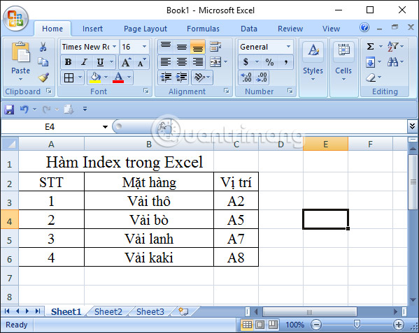
Excel Table 1 : We have a list of fabric types. Find the name of the fabric type knowing that it is in row 2, column 2.

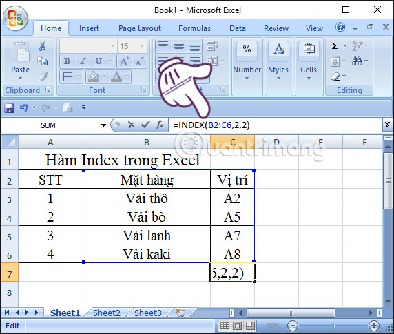
In cell C7, enter the formula above using the syntax below, and then press Enter to execute the Index function.

=INDEX(B2:C6,2,2)

 

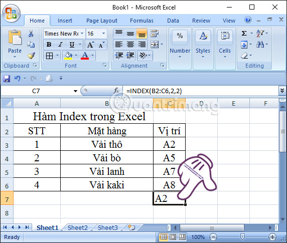
Immediately afterwards, we will be returned the value of position A2 corresponding to the item type Raw Fabric.

2. Excel Index function by reference

The Index by Reference function returns a reference to the cell located at the intersection of a specific row and column. The formula for Index by Reference is as follows:

=INDEX(Reference,Row_num,[Column_num],[Area_num])

In there:

1. Reference : a required reference area.
2. Row_num : the row index from which to return a reference, required.
3. Column_num : the column index from which to return a reference, optionally.
4. Area_num : the number of the cell range to which the value in Reference will be returned. If Area_num is omitted, the INDEX function uses range 1, optionally.

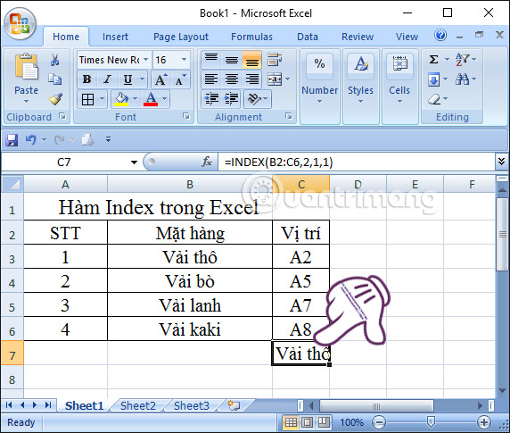
Using the same Excel data table as above, we enter the formula as below. Then press Enter. Click on cell C7 and enter the following formula:

=INDEX(B2:C6,2,1,1)

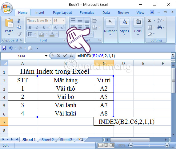
The result will be the name of the item type "Raw Fabric" in line B2.

 

Things to note

1. After the reference and area_num have selected a specific range, row_num and column_num select a specific cell: row_num 1 is the first row in the range, column_num 1 is the first column, etc. The reference returned by INDEX is the intersection of row_num and column_num.
2. If row_num or column_num is set to 0, INDEX returns a reference to the entire column or row, respectively.
3. Row_num, column_num, and area_num must point to a cell in the reference; otherwise, INDEX returns a #REF error. If row_num and column_num are omitted, INDEX returns the area in the reference specified by area_num.
4. The result of the INDEX function is a reference and is interpreted as such by other formulas. Depending on the formula, the return value of INDEX can be used as a reference or a value. For example, the formula CELL("width",INDEX(A1:B2,1,2)) is equivalent to CELL("width",B1). The CELL function uses the return value of INDEX as a cell reference. In other words, a formula like 2*INDEX(A1:B2,1,2) converts the return value of INDEX into a number in cell B1.

In summary, we have guided you on how to use the INDEX function in both array and reference form. The INDEX function can reference any cell in Excel, and the process is not too difficult. You can use this function in combination with other Excel functions for more efficient use in spreadsheet data.

To perform data calculations and create statistical tables in Excel more easily and quickly, you should also know Excel shortcuts or how to handle Excel files when problems arise .

Please refer to the following articles for more information:

1. A compilation of valuable keyboard shortcuts in Microsoft Excel.
2. You want to print text and data from Microsoft Excel. It's not as simple as Word or PDF! Read on!
3. 10 ways to recover corrupted Excel files

Good luck with your project!