How to use Vlookup function in Excel to search and reference

If you are new to Excel, working with data can be daunting. Learn how to use the VLOOKUP function to improve your Excel skills with Free Download.

How to use Vlookup function in Excel to search and reference Picture 1

What is Vlookup? Formula and examples

Quick view:
I. What is the Vlookup function?
II. Vlookup function syntax
III. Examples of the Vlookup lookup function
IV. How to combine Vlookup with Hlookup, Left, Right, Match
V. Common errors when using the Vlookup function.

I. What is the Vlookup function?

VLOOKUP is a basic and popular function in Excel, allowing users to search for data by column. You can quickly look up and get the desired results with just a few steps.
 

II. Vlookup function syntax

In there:

- lookup_value: The value to look up.

-  table_array: Table of values ​​to look up, set in Absolute address form (with $ sign in front by pressing F4).

-  col_index_num: The order of the column to get data from in the lookup value table.

-  range_lookup: Search range, TRUE is equivalent to 1 (relative search), FALSE is equivalent to 0 (absolute search).
 

III. Example of Vlookup function in Excel

With Vlookup's relative and absolute search, you can easily count data on Excel spreadsheets. Vlookup helps you count details to make reports and filter out necessary lists, making your work more accurate and less time-consuming.
 

1. Use Vlookup to search relatively

Example: Based on the classification table corresponding to the given scores, classify the academic performance of the students listed below:

How to use Vlookup function in Excel to search and reference Picture 2

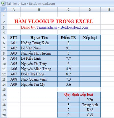
Excel Vlookup function example

We use the formula in column D6: =VLOOKUP(C6,$C$16:$D$20,2,1)
The result is:

How to use Vlookup function in Excel to search and reference Picture 3

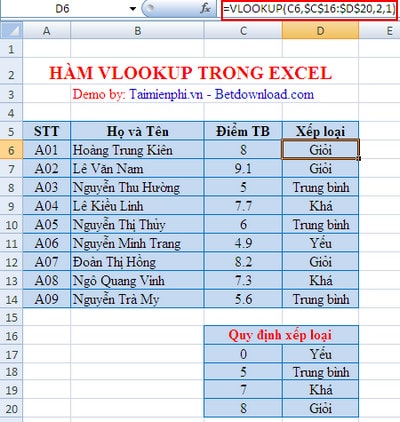
Results when using vlookup function
 

2. Use Vlookup for absolute search

With absolute search, you will find more details than relative search.
For example: Fill in the information of the Hometown and qualifications of the employees in the table based on the corresponding employee code given below.

How to use Vlookup function in Excel to search and reference Picture 4

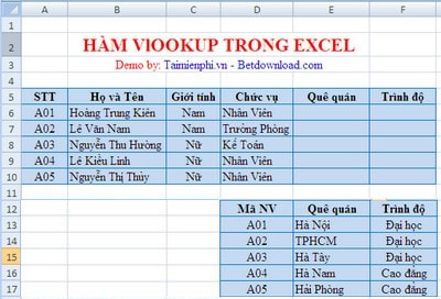
Absolute search example when using vlookup function

To fill in the employee's hometown information, we use the Vlookup formula for cell E6 as follows: =VLOOKUP(A6,$D$12:$F$17,2,0)
A6 is the value to look up
$D$12:$F$17 is the lookup table
2 : data column number on the lookup table
0 : Exact lookup type

How to use Vlookup function in Excel to search and reference Picture 5

Similarly, to fill in the employee's qualifications box, we do the following:

With cell F6 has the formula: =VLOOKUP(A6,$D$12:$F$17,3,0)

How to use Vlookup function in Excel to search and reference Picture 6

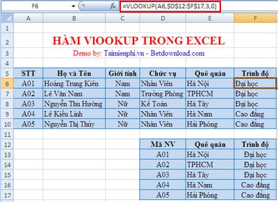
Results of using Vlookup function to find absolute value

3. Relative value and absolute value of Vlookup

With absolute values, you will find the most accurate results, absolute values ​​will not change addresses even if they appear in new columns and cells. Therefore, we use absolute values ​​in cases where we need to find the most accurate information and use relative values ​​in cases where we need to find the most accurate, most accurate results. To learn more, readers can refer to the article on referencing functions in Excel .

IV. How to combine Vlookup with Hlookup, Left, Right, Match

In the above content, Free Download has guided you to learn the basics of the Vlookup function. To help you understand better and apply it more practically, we will now give a specific exercise situation as follows. This problem is a combination of the Vlookup function and functions in Excel such as the Hlookup function or the Left function, the Right function and the Match function.

Given data as in the table below with the following convention:
- Table 1: RICE CONSUMPTION STATISTICS TABLE
- Table 2: TABLE OF PRODUCT NAME, MANUFACTURER NAME AND UNIT PRICE

How to use Vlookup function in Excel to search and reference Picture 7

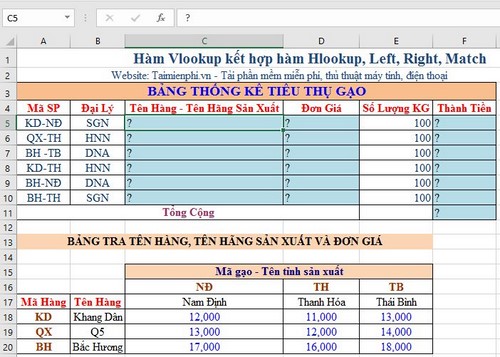
Requirements to be solved:

Question 1: Based on the 2 characters on the left and 2 characters on the right of the Product Code in Table 1, look up in Table 2 to fill in the value for the Item Name - Manufacturer Name columns (Calculate data for columns C5:C10).
Example: KD-ND means Khang Dan rice - Nam Dinh.
Question 2: Fill in the Unit Price for each item based on the Product Code in Table 1 and look up in Table 2. (Calculate data for columns D5:D10).
Question 3: Calculate the total amount = Quantity * Unit price

Answer:

Question 1:
- Explanation: We need to come up with a formula to get the data of Product Name and Production Province Name, then combine these two calculation formulas to get the answer to Question 1.

 + Get the Item Name: Get the 2 characters on the left in the Product Code column in Table 1 (A5:A10) compared to the 2 characters in the Item Code column in Table 2, but the data area we get is also in the Item Name column in Table 2 (A15:B20) or (A15:E20).
 >> We use the Vlookup function: In a cell that has no data, try entering the following formula: =VLOOKUP(LEFT(A5,2),$A$15:$B$20,2,FALSE)
After entering, press Enter, if the word "Khang Dan" appears, it means you have completed 40% of the answer to Question 1, simple right? Let's continue.

+ Get the Production Province Name: Get the 2 characters on the right in the SP Code column (A5:A10) in Table 1 compared with the 2 characters in the "Row" Rice Code - Production Province Name in Table 2, the data area will be (A16:E20).
 >> Get data compared by row, so we use the Hlookup function. Also in a cell with no data, try entering the following formula:

= HLOOKUP(RIGHT(A5,2),$C$16:$E$20,2,FALSE)
After entering, you also continue to press Enter, if the word "Nam Dinh" comes out, it means you have completed 40% of the answer to Question 1. Now you have figured out the answer, right? The next job is to combine these 2 functions to calculate the data in the column Product Name - Production Province Name

+ Combine 2 formulas: There are many formulas to combine or concatenate strings together. In this problem, Free Download will guide you on how to combine strings using the & function. In this problem, we will use a hyphen (with a space) to separate the two formulas that have calculated the results before, that is, the Product Name and the Production Province Name, specifically: " - "
 In general, the function will be as follows =+vlookup&" - "&hlookup (No more = sign at the beginning of the Hlookup function)
 At that time, at C5, you enter the formula:
 C5=+VLOOKUP(LEFT(A5,2),$A$15:$B$20,2,FALSE)&" - "&HLOOKUP(RIGHT(A5,2),$C$16:$E$20,2,FALSE)
 Press Enter to see the result, If the answer is correct, it must be "Khang Dan - Nam Dinh"
 The result is ok, in the next cell is C6:C10, you just need to point the mouse next to the formula in cell C5 and drag it down to C10, and you're done
 . Similarly,

C6=+VLOOKUP(LEFT(A6,2),$A$15:$B$20,2,FALSE)&" - "&HLOOKUP(RIGHT(A6,2),$C$16:$E$20,2,FALSE)
That's it, Question 1 of the given problem is done, let's continue to answer Question 2, guys.

Question 2: Calculate Unit Price The formula
will be as follows: In cell D5, enter the formula
D5=+VLOOKUP(LEFT(A5,2),$A$16:$E$20,MATCH(RIGHT(A5,2),$A$16:$E$16,0),FALSE)

Question 3: Calculate the total amount
Oh, this question often appears in data calculation problems such as payroll, costs, total amount, . Quite easy, right?
The formula to calculate the total amount will be as follows, In cell F5, enter E5=+D5*E5

V. Common errors when using the Vlookup function

1. Error #N/A

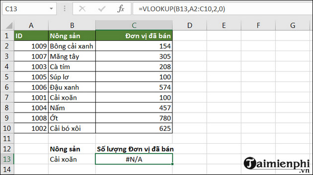
What is #NA error?  #NA error is returned in excel formula when no matching value is found. When using Vlookup, we get #NA error when the search condition is not found in the control area, exactly here is the first column in the condition area of ​​this function.

How to use Vlookup function in Excel to search and reference Picture 8
 

2. #REF! Error

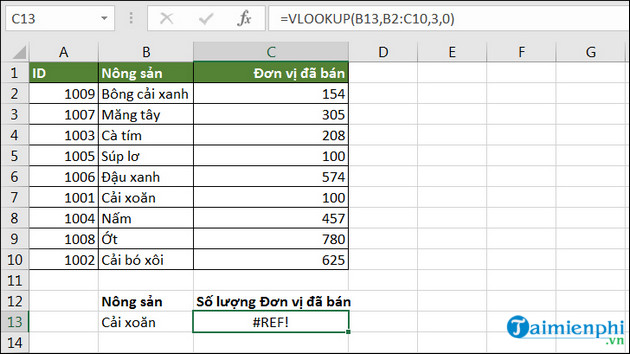
#REF! error occurs when the column being indexed is not defined, for example in the article below  Col_index_num is 3 , while Table_array is B2:C10 which has only 2 columns. Therefore the system will report #REF! error.

How to use Vlookup function in Excel to search and reference Picture 9
 

3. #VALUE! Error

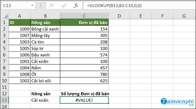
The #VALUE! error occurs when the  Col_index_num column is less than 1 in the formula. For example, in the article below,  Col_index_num is 0, which results in the #VALUE! error.

How to use Vlookup function in Excel to search and reference Picture 10
 

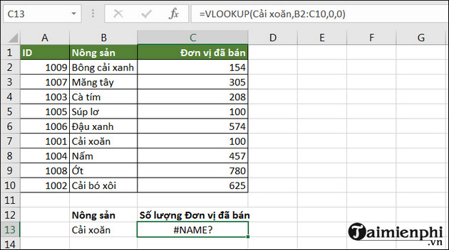
4. #NAME error?

The #NAME? error  occurs when Lookup_value is missing a double quotation mark ("") (the "" is used to format text to help Excel understand the formula). In the example below, Kale is missing a double quotation mark (""), which makes Excel unable to understand the formula.  Fix the error by replacing Kale with "Cải Kale" .

How to use Vlookup function in Excel to search and reference Picture 11

VI. Some notes when using the VLOOKUP function

1. Use absolute references

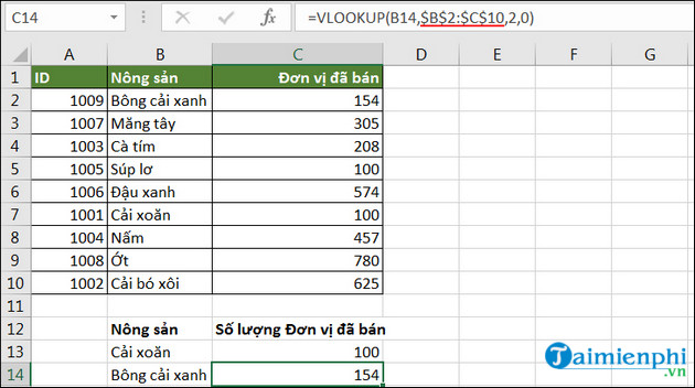
Using absolute references helps you copy formulas from one column to another without changing them.

As in the example below, we have the formula in cell C13 as =VLOOKUP(B13,$B$2:$C$10,2,0) . When copying the formula to cell C14, Table_array will remain the same.

How to use Vlookup function in Excel to search and reference Picture 12
 

2. Do not save numeric values ​​as text

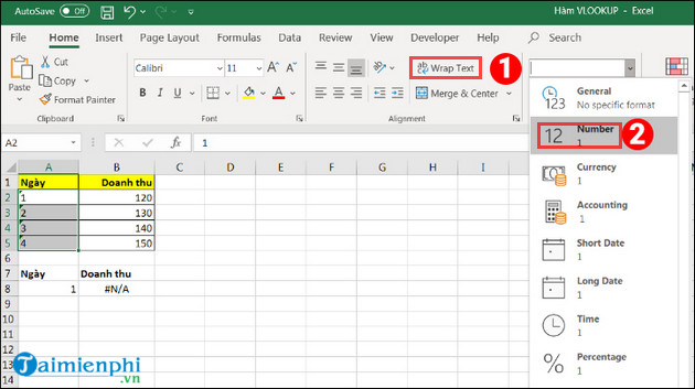
If the numeric data in the data table is in text format as in the example below of column A. When you enter the formula =VLOOKUP(A8$A$2:$B$5,2,0) in the revenue column, the data will return the #N/A error. To convert text data to numbers, simply select Home => Select Wrap Text => Select Number .

How to use Vlookup function in Excel to search and reference Picture 13
 

3. The lookup table contains duplicate values

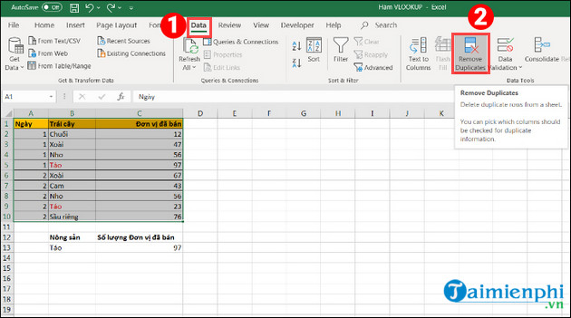
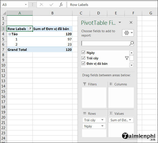
If your table contains multiple duplicate values, VLOOKUP will return the first result it finds from top to bottom. For example, the table below returns Apples as 97 instead of 23.

How to use Vlookup function in Excel to search and reference Picture 14

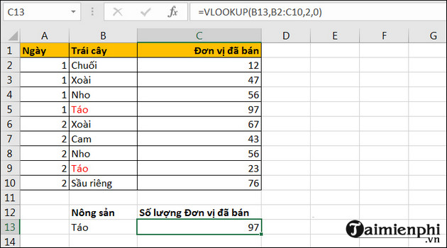
- Solution 1: If you want to remove duplicate values, highlight the lookup table and select Data  => Select  Remove Duplicates

How to use Vlookup function in Excel to search and reference Picture 15

- Solution 2: Use Pivot Table to filter the result list

How to use Vlookup function in Excel to search and reference Picture 16

In Excel, Vlookup is commonly used to help you search for values ​​and return results quickly. Currently, you can apply one of two ways to search for the Vlookup function, which are relative search and absolute search.

Besides Vlookup, there are many other calculation functions in Excel. And the SUMIF function is one of the most used functions, combining the IF function and the Sum function, helping you calculate the total of individual columns and rows without having to calculate the total of all data in the Excel file.

In addition, Excel users cannot ignore the MID function, this is a basic function in Excel that supports cutting character strings in a given character range in a spreadsheet. The MID function is used a lot in cases where it is necessary to extract the most special characters in long character strings that can be up to hundreds of characters.

Jessica Tanner

Update 09 December 2024