How to link data between spreadsheets in Google Sheets

Most of us are familiar with basic operations when using spreadsheets in Google Sheets like using specific rows and columns, calculating, creating pie charts, columns, lines from data, etc. But Why do we just stop there. You need to improve spreadsheets like linking data between spreadsheets, taking data or ranges of data accurately and putting them in a completely new position on another sheet. So this article will show you how to link data using QUERY and IMPORTRANGE functions.

1. How to set up the right to edit spreadsheets on Google Sheets

Note : When linking data to another spreadsheet, you need to click on the box and " Allow Access " after entering the formula, otherwise the data will not appear.

How to link data using the IMPORTRANGE function

The first, most basic method for linking data between spreadsheets is to use the IMPORTRANGE function. Here is the syntax:

= IMPORTRANGE ("spreadsheet_key", "range_string")

"Spreadsheet key" is a long string of numbers and letters in the URL for a given spreadsheet. "Range string" is the exact name of the spreadsheet that takes data (called "Sheet1", "Sheet2", etc. . by default), followed by '!' and the range of cells that want to retrieve data.

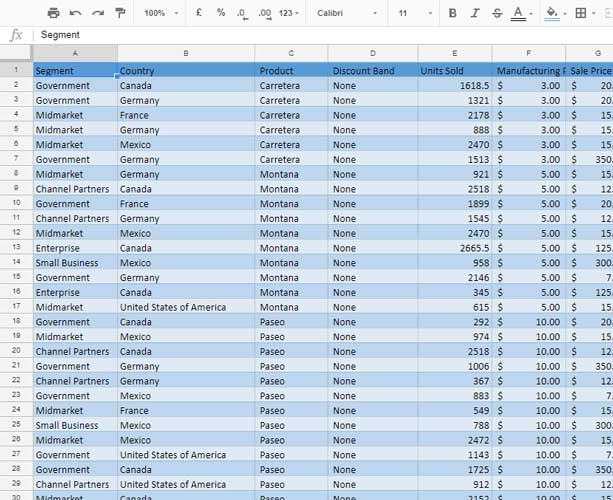
Below is the table that will link the data:

On this spreadsheet, we will get the data from cell A1 to D100. Therefore we will have the following formula:

= ImportRange ("1ByTut9xooZdPIBF55gzQ0Cdi04owDTtLVc_gPGtOKY0", "Sheet1! A1: D100")

This formula will import data from a spreadsheet to another spreadsheet. Here is the data from cell A1 to D100 from the worksheet "Sheet1". The data that will be displayed to another spreadsheet remains the same format as in the original sheet.

Use the QUERY function to enter conditional data

The IMPORTRANGE function is used to transfer data in bulk between worksheets, but if you want to link specific data, use the Query function. This will search for certain words or conditions you have set, then drag the corresponding data from the same row or column.

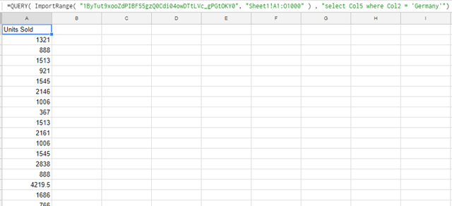
For example, here we will get the German 'Units Sold' data.

To get data type the following formula:

= QUERY (ImportRange ("1ByTut9xooZdPIBF55gzQ0Cdi04owDTtLVc_gPGtOKY0", "Sheet1! A1: O1000"), "select Col5 where Col2 = 'Germany'")

Here, "ImportRange" data follows the previous syntax correctly and then we will specify the function to column 5 as the column "Units Sold" containing column 2 'Germany'. Therefore, there are two "arguments" in this query that are ImportRange and select ColX where ColY = 'Z'.

The above instructions allow you to create links between spreadsheets and can update data automatically when changing on a spreadsheet.

I wish you all success

See more:

1. List of common shortcuts for Google Sheets on computers (Part 1)
2. 6 useful functions in Google Sheets you may not know yet
3. Tricks using Google Sheets should not be ignored