How to Fix Formulas in Excel, Fix Data Ranges in Excel

This guide explains how to resolve Formulas in Excel, Fix Data Ranges, starting with the most likely causes and moving through practical troubleshooting steps.

To fix formulas or ranges in Excel, use the absolute address or use the $ sign in the cell address to fix.

In a cell address that includes column and row indexes, you want to freeze the row or column you just need to lock the value of the corresponding cell address.

1. Fix any value in the formula

For example, the following table needs to calculate the amount to be paid to a level 1 agent. The amount to be paid will be equal to the quantity value in column B times the unit price in cell C5. If you only enter the formula = B5 * C5:

When you press Enter you will see that the value is only true in cell C7 when copying the formula for other cells you will see that there will be cells that receive the wrong value:

The reason the formula will be wrong for the following cells is because the multiplication unit formula is fixed to cell C5, in the formula B5 * C5 in absolute form, so when copying the formula for values other than cell C5 is changed follow, for example here cell C6 has no numeric value so the value returns a Value error:

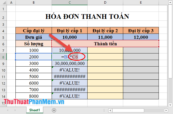
- So with this formula and problem you need to fix the unit price value in cell C5. Because the card request is only charged for a tier 1 agency, you can:

+ Fix row 5 of cell C5: C $ 5.

+ Or freeze both row 5 and column C of cell C5: $ C $ 5.

- You just need to click on the formula to press F4 key 1 time to be able to change C4 addresses into absolute addresses (fixed columns and rows):

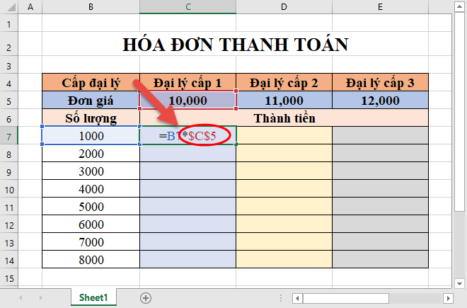
- With the requirement to only charge a first-class agent, so you can only fix row 5 without fixing column C, you just need to press F4 key 2 to fix row 5:

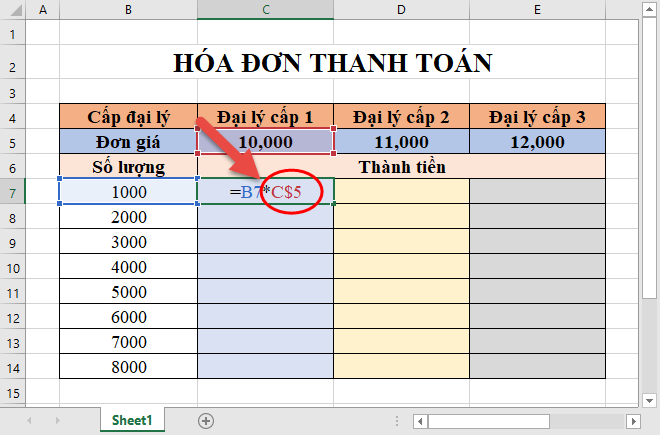
- With the two fixed ways above, give the right results when you charge the agent level 1:

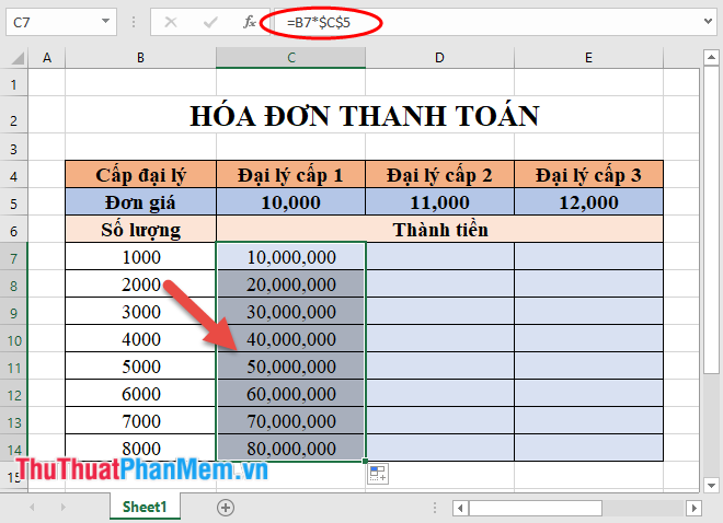
- You note when pressing the F4 key 3 times we switch to fixed column C without fixing the 5th row of C5:

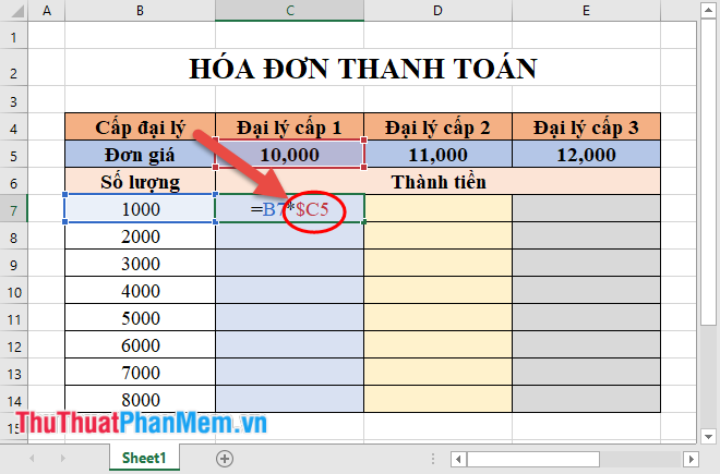
- And so the calculation results will return the wrong value:

2. Fixed the values in the formula

- With the calculation as in part 1, you have charged the money to the level 1 agent. With the level 2 and 3 agents, you can do the same thing. But that calculation is not optimal, in this article TipsMake. com will introduce you how to calculate quickly by fixing data.

- The maths set out the money for agents at all levels with each agent has a different unit price.

- Analysis of problems

+ The general formula to calculate the money for 3 agents: Bx * K5.

In which: x runs from 7 to n is the row, K is the column corresponding to agents with K equal to 1 of 3 values C, D, E.

=> So in the formula the value changes will be: x of the row value of the address Bx and K is the column value of the address K5. Fixed values are column B and row values 5.

=> In the formula you need to fix column B, and row 5 of K => get the absolute address of column B and row 5:

Step 1: Fix column B of B7.

In the cell to calculate the amount of money of first-class agents enter the formula = B7 => perform press F4 three times (pressing F4 times 1 will fix both rows and columns of B7, press F4 times 2 to fix row 7 of B7, press F4 3 times to fix column B of B7):

Step 2: Fix row 5 of K5.

Continue to press the multiplication sign of the operation -> click on the value of cell C5 -> press F4 twice you lock the row of the unit address:

Step 3: Press Enter to get the results.

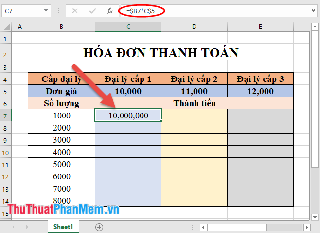
Step 4: Copy the formula for the values in the dealer level column 1 to be the result.

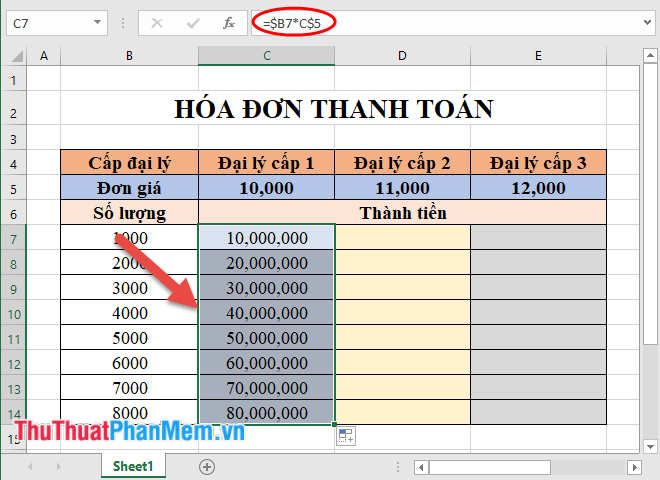
Step 5: When dragging to the last cell value of the dealer column of level 1, keep clicking and drag to the right for agents of level 2 and level 3 to get the results.

You can double check the results, there will certainly be no false values. By doing this, you have reduced the number of formula creation times to agents at level 2 and level 3. So you pay attention to how to fix the data using the absolute address and depending on the value to fix the column. And every row you can lock them easily.

For each cell address, press F4 key to fix data as follows:

- Press F4 times 1: Freeze both rows and columns of the corresponding cell address.

- Press F4 twice: Fixed row value of the corresponding cell address.

- Press F4 times 3: Fixed column values of the corresponding cell addresses.

The above is a way to fix the formula or fix the range of data in a formula in Excel. Good luck!