You already know the SUMIF function to calculate conditional sum in Excel, but you do not know how to use the SUMIF function with 2 or more conditions in Excel. So you let TipsMake.com find out in this article.

Here TipsMake.com share to you how to use the SUMIFS function with 2 or more conditions in Excel, please follow along.
The SUMIF function is a function that sums 1 condition.If you want to sum with 2 or more conditions in Excel, you need to use the SUMIFS function.
Syntax of SUMIFS function:
= SUMIFS (sum_range, criteria_range1, criteria1, [criteria_range2, criteria2], .)
Inside:
- Sum_range : a required argument, this is the range of cells to sum.
- Criteria_range1 : is a required argument, this is the range to be tested using Criteria1 .
- Criteria1 : required argument, this is the condition that identifies a cell within Criteria_range1 .
Criteria_range1 and Criteria1 are set as a search pair, whereby a range is searched according to specific criteria.
- Criteria_range2, Criteria2 . are optional arguments, these are additional ranges and conditions associated with the argument. The SUMIFS function supports up to 127 range of conditions / conditions.
For example , using the SUMIFS function with 2 or more conditions in Excel.
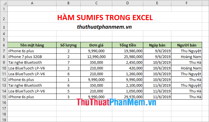
Suppose you have the data table as shown below:

Because of the total sale proceeds, Sum_range is the total sum column D7: D15 .
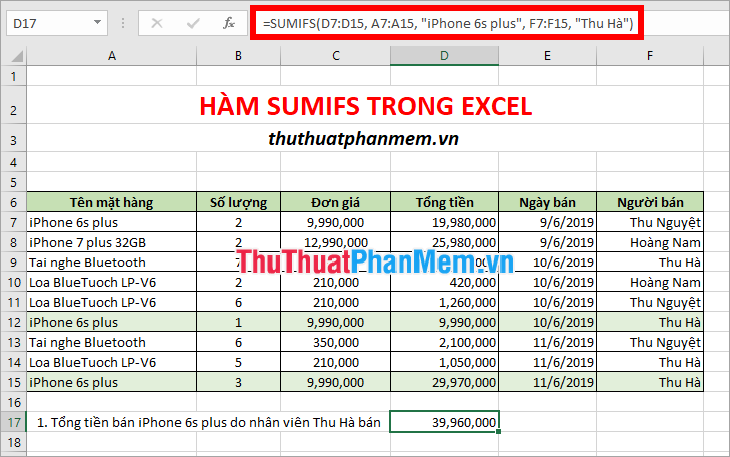
According to this requirement, the SUMIFS function will have 2 pairs of range / condition:
- Scope 1 is A7: A15 with condition 1 is "iPhone 6s plus"
- Scope 2 is F7: F15, provided that condition 2 is "Thu Hà"
Thus, the SUMIFS function will look like this:
= SUMIFS (D7: D15, A7: A15, "iPhone 6s plus", F7: F15, "Thu Ha")

Because of the total sale, Sum_range is D7: D15
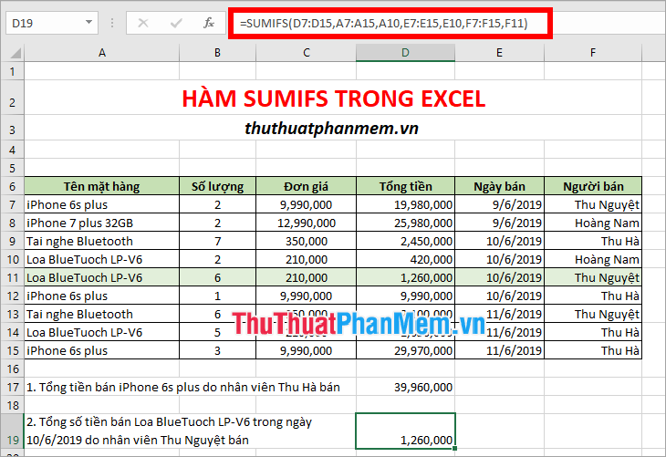
This requirement has 3 conditions with the following range / condition pairs:
- Range 1 is A7: A15, provided that the "BlueTuoch LP-V6 Speaker"
- Range 2 is E7: E15 provided that "June 10, 2019"
- Range 3 is F7: F15 provided that "Thu Nguyet"
Thus the SUMIFS function syntax is as follows:
= SUMIFS (D7: D15, A7: A15, A10 , E7: E15, E10 , F7: F15, F11 )

Above TipsMake.com showed you how to use the SUMIFS function with 2 or more conditions in Excel. Hopefully through this article, you will better understand the SUMIFS function in Excel to use summing when two or more conditions are required. Good luck!


 How to combine Vlookup function with Left function
  Techniques to exploit buffer overflows: Organize memory, stack, call functions, shellcode
  How to use the SWITCH function in Excel 2016
  Differentiate between SUM, SUMIF, SUMIFS and DSUM functions
  Instructions for using the IF function in Excel
  How to combine Sumif and Vlookup functions in Excel