How to use the XLOOKUP function in Excel?

Excel's new XLOOKUP function replaces VLOOKUP, which provides a powerful replacement for one of Excel's most popular functions. This new function addresses some of the limitations of VLOOKUP and adds other functions. This article will guide you how to use this new XLOOKUP function.

1. How to use the Search function in Excel?
2. How to combine Sumif and Vlookup functions in Excel?
3. How to use the Lookup function in Excel?

What is XLOOKUP?

The new XLOOKUP function is the solution to some of VLOOKUP's major limitations. It also replaces the HLOOKUP function. For example, XLOOKUP can look to the left, default to find exact results, and allow specifying cell ranges instead of column numbers. VLOOKUP is not easy to use and inflexible.

Currently, XLOOKUP is only available to Insiders users. Anyone who participates in the Insider program can access the latest Excel feature as it becomes available. Microsoft will soon release this function to all Office 365 users.

How to use the XLOOKUP function?

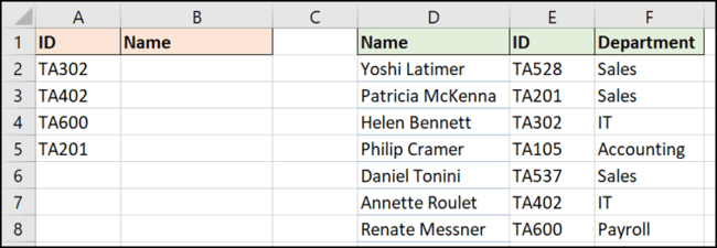
See the example below to understand how XLOOKUP works. In this example, we need to return the element from column F for each ID in column A.

How to use the XLOOKUP function in Excel? Picture 1

This is an example of finding an exact result, but the XLOOKUP function requires only three types of information.

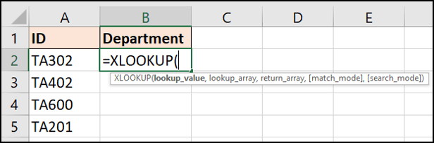
The image below shows XLOOKUP with 5 arguments, but the first three need exact results. So focus on them:

1. Lookup_value : Search value
2. Lookup_array : Search range
3. Return_array : Range contains the value to return

How to use the XLOOKUP function in Excel? Picture 2

In this example, we will use the formula:

 =XLOOKUP(A2,$E$2:$E$8,$F$2:$F$8) 

How to use the XLOOKUP function in Excel? Picture 3

Now let's explore some advantages of XLOOKUP over VLOOKUP.

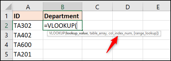
No more index column numbers

The third argument of VLOOKUP is to specify the number of columns of information to be returned from the table range. This is no longer an issue with XLOOKUP because this function allows the user to select a return range. (column F in this example).

How to use the XLOOKUP function in Excel? Picture 4

And don't forget, XLOOKUP can view the remaining data of the selected cell, unlike VLOOKUP.

You also do not have the problem of formula errors when adding new columns. If this happens in a spreadsheet, the range returned will be adjusted automatically.

How to use the XLOOKUP function in Excel? Picture 5

Absolute match by default

When using VLOOKUP, the user must specify an absolute match if desired. But with XLOOKUP, the default is absolute match. This helps reduce the fourth argument and ensures new users are less likely to make mistakes. In a nutshell, XLOOKUP requires fewer questions than VLOOKUP and is user friendly.

XLOOKUP can look on the left

The ability to select the lookup range makes XLOOKUP more flexible than VLOOKUP. With XLOOKUP, the order of the columns in the table doesn't matter.

VLOOKUP is restricted by searching the leftmost column of the table and then returning from a specified number of columns to the right.

In the example below, we need to look up the ID (column E) and return the person's name (column D).

How to use the XLOOKUP function in Excel? Picture 6

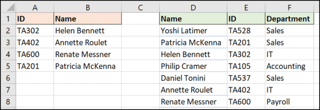
Use the formula below:

 =XLOOKUP(A2,$E$2:$E$8,$D$2:$D$8) 

How to use the XLOOKUP function in Excel? Picture 7

Use XLOOKUP to search the range

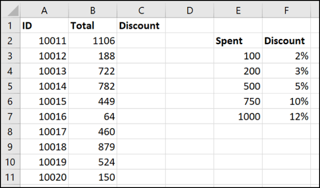
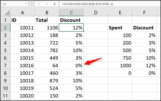
Although not as common as absolute matches, you can use a search formula to find a value in the range. For example, we want to return a discount depending on the amount spent.

This time we don't look for a specific value and need to know which range in the column B values ​​in column E to determine the discount.

How to use the XLOOKUP function in Excel? Picture 8

XLOOKUP has an optional fourth argument (remember, it defaults to an absolute match) called match_mode.

How to use the XLOOKUP function in Excel? Picture 9

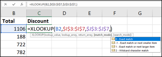
You may find that XLOOKUP can find approximate results better than VLOOKUP.

There is option to find the closest match less than (-1) or the closest greater than (1) search value. There is also an option to use wildcards (2), such as? or *. This setting is not enabled by default as with VLOOKUP.

The formula in this example returns the closest value smaller than the search value if no exact match is found:

 =XLOOKUP(B2,$E$3:$E$7,$F$3:$F$7,-1) 

How to use the XLOOKUP function in Excel? Picture 10

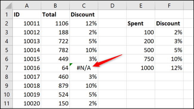
However, there was an error in cell C7, which should have returned the 0% discount because only spent 64, did not meet the criteria to receive the discount.

Another advantage of the XLOOKUP function is that it does not require the scope to search in ascending order like VLOOKUP.

Enter a new row at the bottom of the lookup table and then open the formula. Expand the scope of use by clicking and dragging the corners.

How to use the XLOOKUP function in Excel? Picture 11

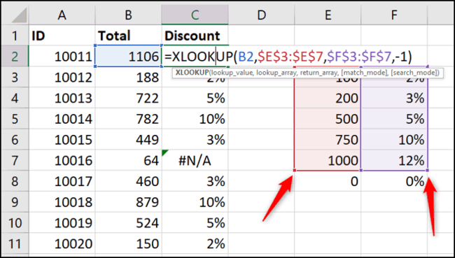
The formula immediately corrects the error. It has no problem with having 0 at the end of the range table.

How to use the XLOOKUP function in Excel? Picture 12

XLOOKUP replaces HLOOKUP

As mentioned, the XLOOKUP function can also replace the HLOOKUP function. A function can replace two functions, nothing is better.

The HLOOKUP function looks up horizontally, which is used to search by row.

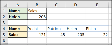
This function is not as well known as VLOOKUP but is useful in cases when the title is in columns A and the data is in rows 4 and 5 as in the example below.

XLOOKUP can be searched in both directions, under columns and along rows.

In this example, the formula is used to return the sales value related to the name in column A2. It looks in row 4 to find the name and returns the value from row 5:

 =XLOOKUP(A2,B4:E4,B5:E5) 

How to use the XLOOKUP function in Excel? Picture 13

XLOOKUP can be viewed from the bottom

Usually you need to look from top to bottom in a list to find the first presence of a value. XLOOKUP has a fifth argument named search_mode. This argument allows the search navigation to start from the bottom up in a list to find the last presence of a value.

In the example below, we need to find the inventory level for each product in column A.

The lookup table is sorted by date order. We want to return inventory from the last inspection (the last occurrence of the Product ID).

How to use the XLOOKUP function in Excel? Picture 14

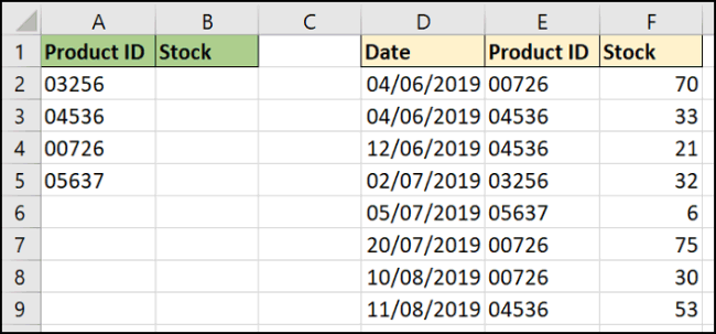
The fifth argument of the XLOOKUP function provides four options. Here we will use the Search last-to-first option .

How to use the XLOOKUP function in Excel? Picture 15

The formula used in this example:

 =XLOOKUP(A2,$E$2:$E$9,$F$2:$F$9,,-1) 

How to use the XLOOKUP function in Excel? Picture 16

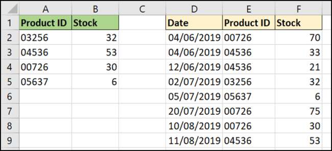
In this formula, the fourth argument is ignored. It is optional and we want the absolute match default.

The XLOOKUP function is the expected successor to both VLOOKUP and HLOOKUP. A series of examples have been used in this article to demonstrate the advantages of the XLOOKUP function.

I wish you successful implementation!