How to use VLOOKUP Function in Excel

What is the VLOOKUP function?

The VLOOKUP function is a built-in function in Excel, classified as a Lookup/Reference Function. It can be used as a workbook function (WS) in Excel. As a worksheet function, the VLOOKUP function can be entered as part of a formula in a worksheet cell.

The VLOOKUP function is actually quite easy to use once you understand how it works!

For example: If you know the name of a product and you want to quickly determine its price, you can simply enter the product name into Excel and VLOOKUP will find the price for you. However, for novice Excel users, setting up VLOOKUP may look like an intimidating process – but it doesn't need to be. Just follow our step-by-step guide on how to use VLOOKUP in Excel today.

How to use VLOOKUP in Excel

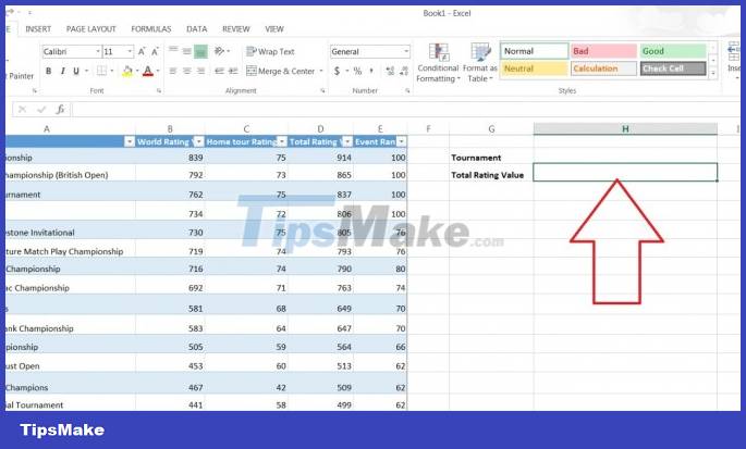
Step 1 . Click the cell where you want to calculate the VLOOKUP formula.

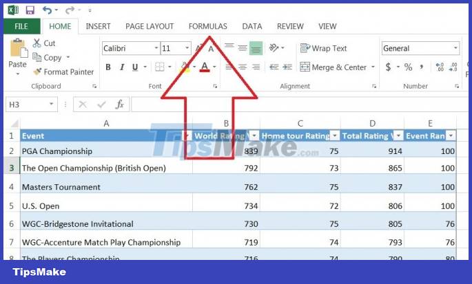
Step 2 . Click ' Formula ' at the top of the screen .

Step 3 .Click ' Lookup & Reference ' on the Ribbon.

Step 4.Click ' VLOOKUP ' at the bottom of the drop-down menu.

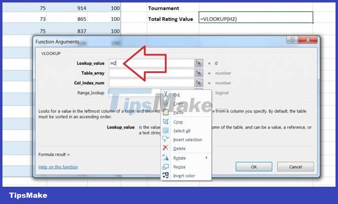
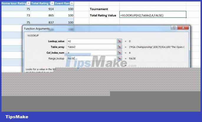
Step 5.Specify the cell   where you will enter the value whose data you are looking for. In this case, our lookup value is H2, as this is where we would enter the name of a tournament, such as 'PGA Championship', so we enter 'H2' in the store's Lookup_value box popup. Once we have VLOOKUP set up properly, Excel will return the Total Rating Value in cell H3 when we enter the tournament name in cell H2.

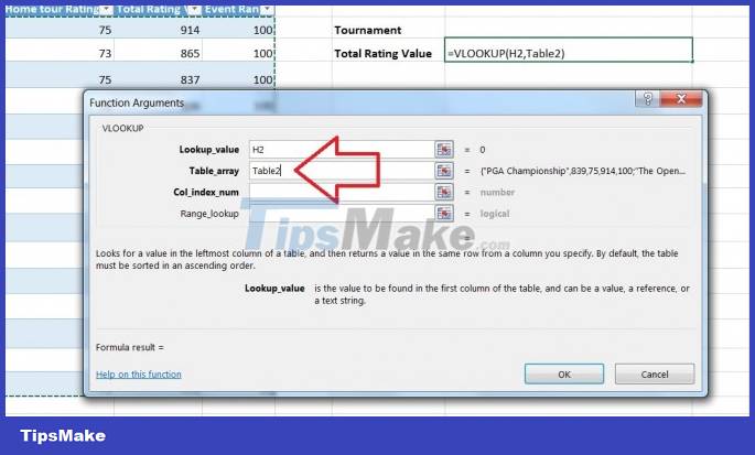
Step 6. Specify the data  that you want VLOOKUP to use for its search in the Table_array box . In this case, we've selected the entire table (not including the headers).

Step 7 .  Specify whether you need an exact match  by entering FALSE (exact match) or TRUE (approximate match) in the Range_lookup box . In this case we want an exact search we enter FALSE .

Step 8 . Click ' OK ' at the bottom of the pop-up window.

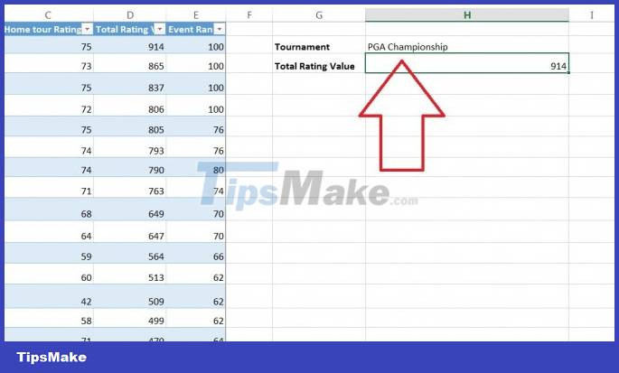
Step 9 . Enter the value   for which data you are looking for. In our example, we want to find the Total Value Rating of the PGA Championship, so we enter 'PGA Championship' in cell H2 and VLOOKUP automatically generates the Total Value Rating (914 in this case) in cell H3 .

Using VLOOKUP , you not only search for individual values ​​but also combine two spreadsheets into one. For example, if you have a spreadsheet with names and phone numbers and another sheet with names and email addresses, you can put the email address next to the name and phone number by using VLOOKUP