How to combine Vlookup function with Left function

In Excel the concept of a combined or nested function is extremely familiar to those who frequently have to process data at a more advanced level, including the Vlookup function combining the Left function. When combining these two functions, the Left function will separate the values ​​to get to the left, then the Vlookup function looks for information that you need to quickly and accurately. The following article will show you how to use Vlookup function with Left function in Excel.

1. How to use Vlookup function in Excel
2. How to combine Sumif and Vlookup functions in Excel
3. Use VLOOKUP to join two Excel tables together

How to find the value using Vlookup function with Left function

Syntax Vlookup function

The function is used to find the value of a certain column.

Function syntax is = VLOOKUP (lookup_value, table_array, col_index_num, [range_lookup] .

Inside:

1. Lookup_value: The value used to search.
2. Table_array: Table of values ​​to detect in the form of absolute address needs a $ sign in front.
3. Col_index_num: The order of the column to retrieve data on the detector value table.
4. Range_lookup: Search range, True or 1 (relative detection), Flase or 0 (absolute detection).

Note , with lookup_value press F4 3 times, for table_array value press F4 1 time.

Using F4 will help you a lot:

1. F4 press 1 time: For absolute value, fix the column and fixed line.
2. F4 presses twice: To have a relative column value and relative line, that is, the line fixation is not fixed.
3. F4 press 3 times: To have relative and absolute column values, that is to fix the column but not to fix the line.

Left function syntax

Left function is used to cut the characters to the left of a character string.

Use function syntax = LEFT (text, n) .

Inside:

1. Text is a string of characters you want to separate.
2. N is the number of characters you want to separate from the left.

For example Vlookup function with Left function

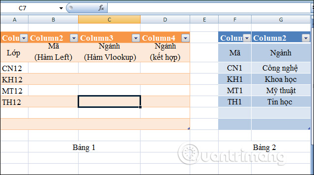
We will do with the data table as shown below.

First of all, we will find out how to use the Left function and Vlookup function on Excel. You will use the Left function to get Sector Code from the Class column.

Step 1:

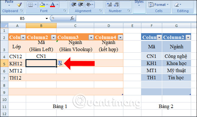
In the Code field cell B4 enter the formula = LEFT (A4.3) to get the 3 characters to the left of cell A4.

Step 2:

Press Enter and we will get the Sector Code character CN1 which is cut from the Class CN12 character string. The industry code in Table 1 is similar to Table 2. At the same time, we will see the character function fx in the cell inserted in the Left formula.

Step 3:

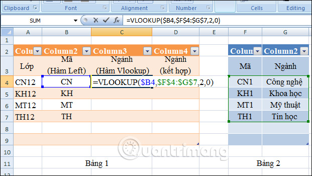
Drag the formula in cell B4 down to the remaining cells, the Left function formula will automatically be copied and the Code Sector result will be automatically filled.

Step 4:

Next to cell C4, enter the Vlookup function formula = VLOOKUP ($ B4, $ F $ 4: $ G $ 7.2,0). Inside:

1. $ B4 is the value used to search in the Industry code column.
2. $ F $ 4: $ G $ 7 is the search data area in Table 2 with the complete Industry Code name.
3. 2 is the order in which the values ​​needed in the data area here are the Sector column in Table 2.
4. 0 is the absolute scope of search.

Step 5:

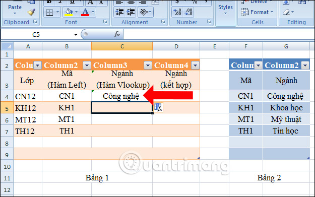
When pressing Enter, the user will get the industry name as Technology corresponding to the established Sector Code.

Step 6:

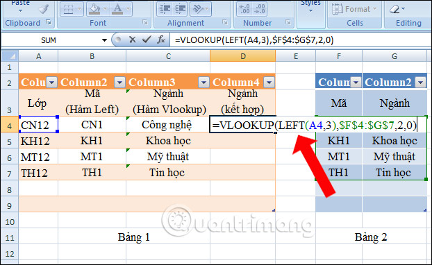
But doing so will take time, we will proceed to combine two functions, Vlookup and Left function together. In cell D4 enter the formula = VLOOKUP (LEFT (A4.3), $ F $ 4: $ G $ 7.2,0) and press Enter.

This means that we will change the value used to search for $ B4 to LEFT (A4.3).

Step 7:

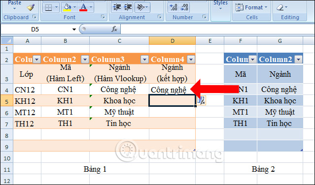
When we press Enter we will also get the result that the Industry name here is Technology.

Finally, you just need to drag down below to complete the branch name is done.

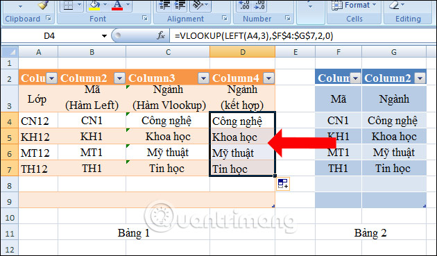
In general, how to combine Vlookup function with Left function in Excel is very simple, you just need to add the Left function with the characters that you want to get from a character area, then localize the data to get the results in vertical rows. With such a combination, we only need to enter the formula once.

See more:

1. How to use PRODUCT function in Excel
2. Simple way to convert Excel files to PDF
3. Function error in Microsoft Excel 2003

I wish you all success!