Excel 2019 (Part 26): Introducing PivotTables

When you have a lot of Excel data , it can sometimes be difficult to analyze all the information in a spreadsheet. PivotTables can help make your spreadsheets more manageable by summarizing the data and allowing you to manipulate it in different ways.

 

Use PivotTables to answer the question.

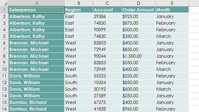
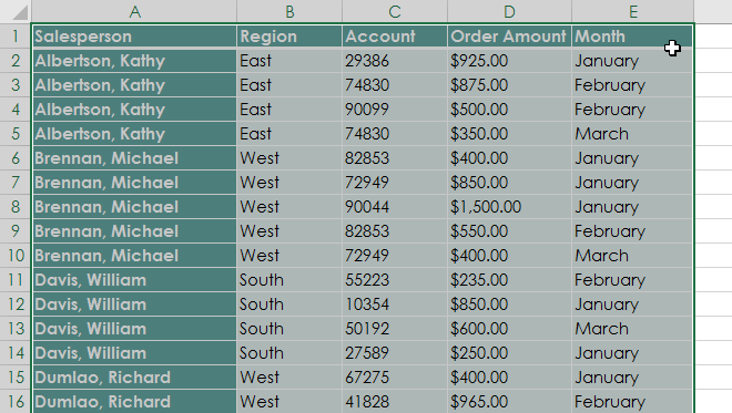
Consider the following example. Suppose you want to answer the question: How many items did each salesperson sell? Finding the answer can be time-consuming and difficult. Each salesperson's name appears on multiple items, and you need to calculate the total of all their different orders. Using the Subtotal command could help find the total for each salesperson, but there's a lot of data to process.

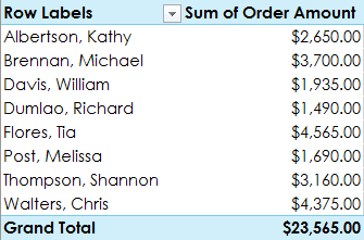
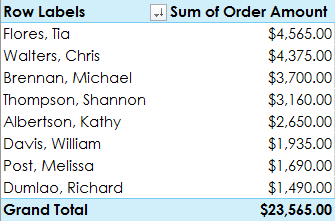
Fortunately, PivotTables can calculate and summarize data instantly in a way that makes it much easier to read. When complete, a PivotTable will look like this:

 

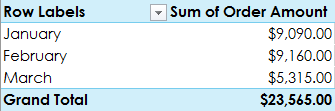
Once you've created a PivotTable, you can use it to answer various questions by rearranging the data. For example, suppose you want to answer: What is the total sales revenue for each month? You can modify the PivotTable as follows:

How to create a PivotTable

1. Select the table or cells (including column headers) you want to include in your PivotTable.

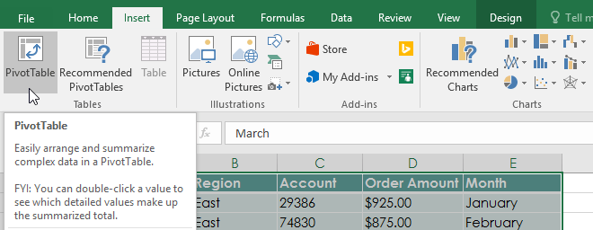
2. From the Insert tab , click the PivotTable command.

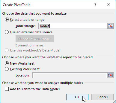
3. The Create PivotTable dialog box will appear. Select your settings, then click OK. The example will use Table1 as the data source and place the PivotTable in a new worksheet.

 

4. Empty PivotTables and Field Lists will appear in a new worksheet.

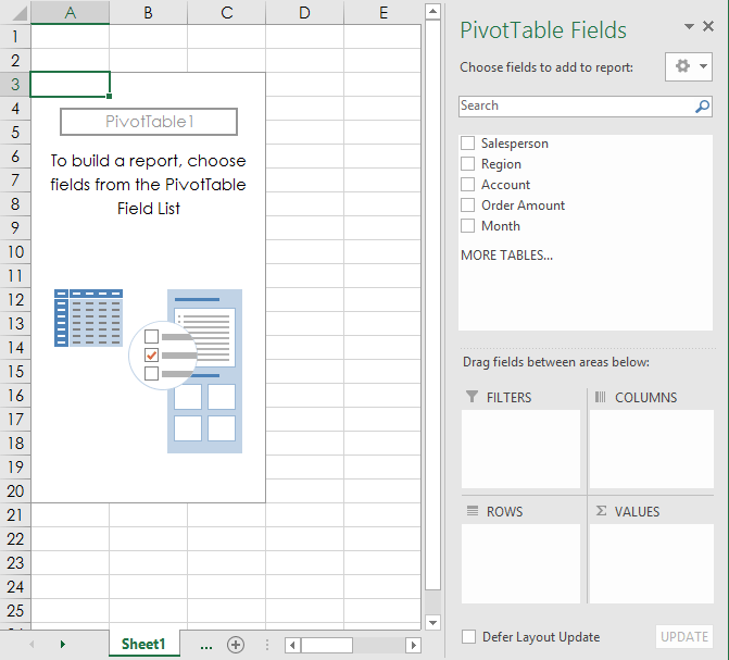
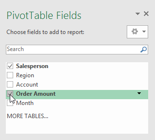
5. After creating the PivotTable, you'll need to decide which fields to add. Each field is simply a column header from the source data. In the PivotTable Fields list , select the checkbox for each field you want to add. For example, if you want to know the total amount sold by each salesperson, the Salesperson and Order Amount fields would be selected.

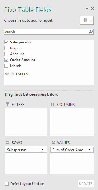
6. The selected fields will be added to one of the four areas below. In the example, the Salesperson field has been added to the Rows area , while Order Amount has been added to Values. You can also drag and drop fields directly into the desired area.

 

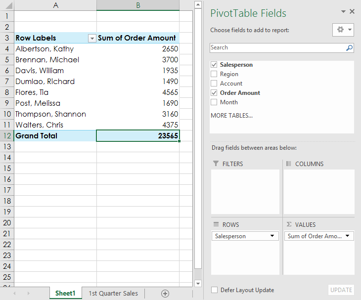
7. The PivotTable will calculate and summarize the selected fields. In this example, the PivotTable displays the number of sales made by each salesperson.

Just like with regular spreadsheets, you can sort data in a PivotTable using the Sort & Filter command on the Home tab. You can also apply any number formatting you want. For example, you might want to change the number format to Currency. However, keep in mind that some formatting may disappear when you modify the PivotTable.

If you change any data in your source worksheet, the PivotTable will not update automatically. To update it manually, select the PivotTable, then go to Analyze > Refresh .

Data rotation

One of the best things about PivotTables is that they can quickly rotate—or reorganize—data, allowing you to examine your spreadsheet in a number of ways. Rotating data can help you answer many different questions and even experiment with the data to discover new trends and patterns.

How to add columns

Until now, PivotTables have only displayed one column of data at a time. To display multiple columns, you need to add fields to the Columns area.

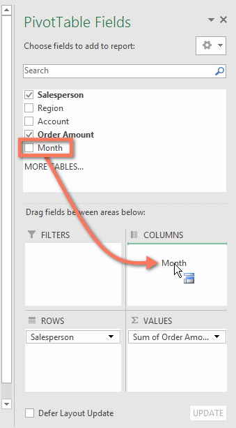
1. Drag a field from the Field List into the Columns area. For example, we'll use the Month field.

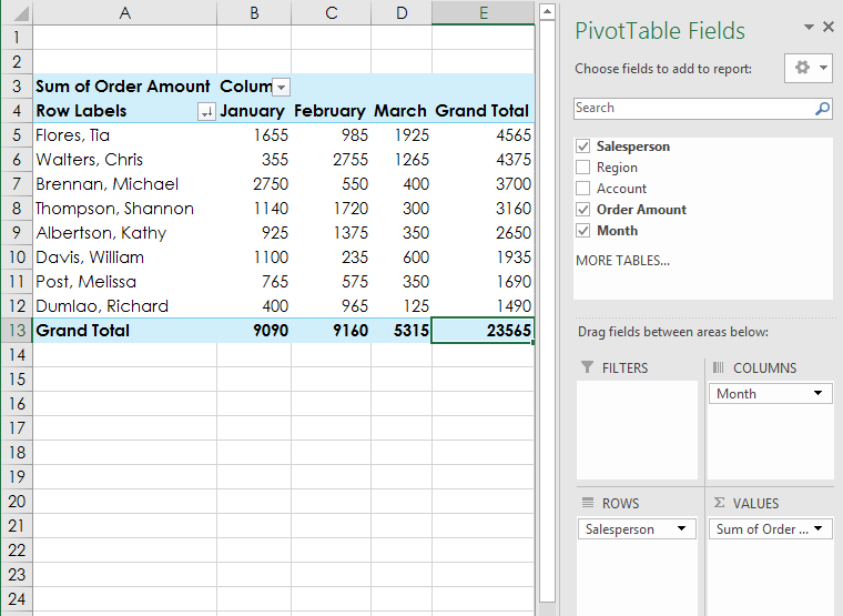
2. The PivotTable will include multiple columns. In this example, there is now a column for each person's monthly sales, in addition to the total.

 

How to change a row or column

Changing a row or column can give you a completely different view of the data. All you have to do is delete the field in question, then replace it with another field.

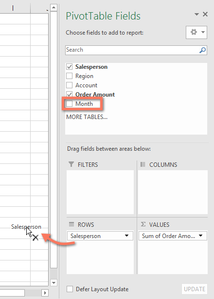
1. Drag the field you want to delete out of its current location. You can also uncheck the appropriate box in the Field List. This example has deleted the Month and Salesperson fields.

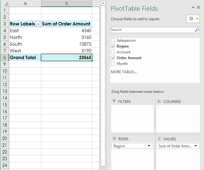
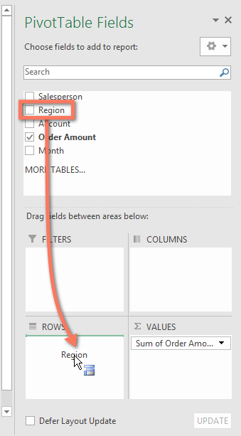
2. Drag a new field into the desired area. For example, this would place the Region field in Rows.

3. The PivotTable will adjust to display the new data. In this example, the number of items sold by region will be displayed.